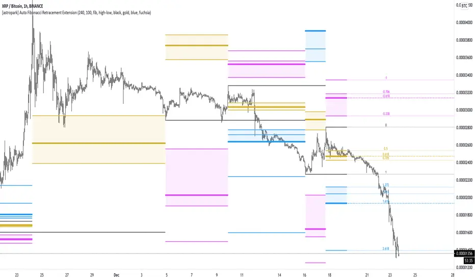
[astropark] Auto Fibonacci Retracement ExtensionDear followers,
today a new analysis tool for day trading, scalping and swing trading: Automatic Fibonacci Retracements and Extensions drawer!
It works on every timeframe and market, as it simply draws automatically most important fibonacci levels on the chart.
Based on the analysis window set (default 100 bars, but you can edit it as you like), it finds recent high and low and start drawing the following levels:
recent high and low (black)
golden retracement range: 0.5 * 0.618 * 0.705 fibonacci retracements (gold)
fibonacci extensions range above 1: 1.272 * 1.424 * 1.618 * 2.618 * 4.236 (blue)
fibonacci extensions range below 0: -0.238 * -0.618 * -0.706 * -1(fuchsia)
Whenever the indicator finds a new high or a new low, al fibonacci levels are re-draw automatically.
The indicator will let you:
change analysis window
enable displaying labels related to current fibonacci levels and/or prices
change colors
show/hide each specific level
How to use the indicator?
Basically, all techniques which apply to fibonacci tool are valid here too.
After a big move up or down, a new high or low is created and a retracement is expected: if trend is strong, retracement to golden ration 0.618 will be a perfect spot for buy or sell respectively in order to continue riding the trend.
In general a bounce is always expected when price hit 0.618 retracement , good to know for scalping traders, while swing trades will continue holding the trade for higher profits.
If the golden retracement range (0.5 - 0.705) is broken and then retested from the other side, a continuation move is expected towards previous high/low (fib level 1) and even more towards the fibonacci extensions range above 1 (1.618 - 2.618 - 4.236).
If the base of bounce and trend continuation on golden retracement range, traders can expect
price to hit again previous high/low and
if trend is strong, a consolidation near the previous high/low range (conditions that are respectively bullish and bearish)
do a further continuation towards -0.618 fib level range
Traders must always understand that
the higher the timeframe, the stronger is the meaning and so the reaction when a specific fibonacci level is hit
don't trade blindly, try to find confluences to have an higher chance to be in a winning trade in near future
money and risk management are very important, so manage your position size and always have a stop loss in your trades
As said, this indicators work on every timeframe and in all markets (Crypto currencies, stocks, FOREX, indexes, commodities). Here some examples:
BTCUSDT 1D: after a long run, a retracement is expected and a bounce at 0.618 golden level is more than obvious: perfect short (sell) entry
BTCUSDT 1D: again as previous example, after a long run, a retracement is expected as well as price's bounces back above
EURUSD 1h: lots of info here, directly in the chart below:
bounces on 0.618 golden zone
double top
price breaks 0.618 level and retests it from below targeting previous low
double bottom and bounce back towards golden zone
bearish consolidation at recent low and further decline towards 1.618 fib extension
AMZN 1h stock: lots of info here too, directly in the chart below:
new high is print, price retrace to golden zone
bounces on 0.618 golden zone
price breaks 0.618 level and retests it from below targeting previous low
double bottom and bounce back towards golden zone
rejection at golden zone, price falling targeting previous low again and probably 1.618 fib extension
price breaks hard previous low and hits fib extension range below recent low
price retraces back up towards new golden retracement range
golden retracement range is broken and used as support: targets are previous high and 1.618 extension
once 1.618 extension level is broken and retested successfully as support, price moves towards 2.618 fibonacci extension level
SPY (SPX500) index: lots of info in the chart
interesting to note that March 2020 huge dump can be totally mapped as a series of fibonacci level bounces, so you understand the importance of riding a trend now, right?
after the low was formed, price retraced perfectly to golden ration 0.618
each time price hit a golden level/range, it retraces creating double top and double bottom configurations too
In the chart below we can see the power of the double bottom at golden retracement level: targets are previous high and -0.618 fibonacci extension level
XAUUSD 15m: as we are in a lower timeframe, the default analysis windows has been reduced to 50.
What can we see here:
golden retracement and price is rejected towards previous low
golden retracement hit and price bounces back lower
new high is formed: golden retracement hit and price bounces back higher
price break previous high and hits fibonacci extensions -0.618 and -1
price continues rising forming a regular bearish divergence with RSI
once uptrend is broken, price falls dramatically
first target is 0.618 retracement level, where you see a very small retracement due to strength of sellers
second target is previous low, which is broken and retested many time from below (bearish retest)
third target is fibonacci extension range (in this case 1.414 is almost hit)
as an hidden bullish divergence with RSI was created, price goes back up
This is a premium indicator , so send me a private message in order to get access to this script.
Cerca negli script per "high low"
Dekidaka-Ashi - Candles And Volume Teaming Up (Again)The introduction of candlestick methods for market price data visualization might be one of the most important events in the history of technical analysis, as it totally changed the way to see a trading chart. Candlestick charts are extremely efficient, as they allow the trader to visualize the opening, high, low and closing price (OHLC) each at the same time, something impossible with a traditional line chart. Candlesticks are also cleaner than bars charts and make a more efficient use of space. Japanese peoples are always better than everyone at an incredible amount of stuff, look at what they made, the candlesticks/renko/kagi/heikin-ashi charts, the Ichimoku, manga, ecchi...
However classical candlesticks only include historical market price data, and won't include other type of data such as volume, which is considered by many investors a key information toward effective financial forecasting as volume is an indicator of trading activity. In order to tackle to this problem solutions where proposed, the most common one being to adapt the width of the candle based on the amount of volume, this method is the most commonly accepted one when it comes to visualizing both volume and OHLC data using candlesticks.
Now why proposing an additional tool for volume data visualization ? Because the classical width approach don't provide usable data regarding volume (as the width is directly related to the volume data). Therefore a new trading tool based on candlesticks that allow the trader to gain access to information about the volume is proposed. The approach is based on rescaling the volume directly to the price without the direct use of user settings. We will also see that this tool allow to create support and resistances as well as providing signals based on a breakout methodology.
Dekidaka-Ashi - Kakatte Koi Yo!
"Dekidaka" (出来高) mean "Volume" in a financial context, while "Ashi" (足) mean "leg" or "bar". In general methods based on candlesticks will have "Ashi" in their name.
Now that the name of the indicator has been explained lets see how it works, the indicator should be overlayed directly to a candlestick chart. The proposed method don't alter the shape of the candlesticks and allow to visualize any information given by the candles. As you can see on the figure below the candle body of the proposed tool only return the border of the candle, this allow to show the high/low wick of the candle.
The body size of the candle is based on two things : the absolute close/open difference, and the volume, if the absolute close/open difference is high and the volume is high then the body of the candle will be clearly visible, if the volume is high but the absolute close/open difference is low, then the body will be less visible. This approach is used because of the rescaling method used, the volume is divided by the sum between the current volume value and the precedent volume value, this rescale the volume in a (0,1) range, this result is multiplied by the absolute close/open difference and added/subtracted to the high/low price. The original approach was based on normalization using the rolling maximum, but this approach would have led to repainting.
You have access to certain settings that can help you obtain a better visualization, the first one being the body size setting, with higher values increasing the body amplitude.
In green body with size 2, in red with size 1. The smooth parameter will smooth the volume data before being used, this allow to create more visible bodies.
Here smooth = 100.
Making Bands From The Dekidaka-Ashi
This tool is made so it output two rescaled volume values, with the highest value being denoted as "Dekidaka-high" and the lowest one as "Dekidaka-low". In order to get bands we must use two moving averages, one using the Dekidaka-high as input and the other one using Dekidaka-low, the body size parameter should be fairly high, therefore i will hide the tool as it could cause trouble visualizing the bands.
Bands with both MA's of period 20 and the body size equal to 20. Larger periods of the MA's will require a larger amount of body size.
Breakout Signals
There is a wide variety of signals that can be made from candles, ones i personally like comes from the HA candles. The proposed tool is no exception and can produce a wide variety of signals. The signals generated are basic ones based on a breakout methodology, here is each signal with their associated label :
Strong Bullish signal "⇈" : The high price cross the Dekidaka-high and the closing price is greater than the opening price
Strong Bearish signal "⇊" : The low price cross the Dekidaka-low and the closing price is lower than the opening price
Weak Bullish signal "↑" : The high price cross the Dekidaka-high and the closing price is lower than the opening price
Weak Bearish signal "↓" : The low price cross the Dekidaka-low and the closing price is greater than the opening price
Uncertain "↕" : The high price cross the Dekidaka-high and the low price cross the the Dekidaka-low
In order to see the signals on the chart check the "Show signals" option. Note that such signals are not based on an advanced study, and even if they are based on a breakout methodology we can see that volatile movement rarely produce signals, therefore signals mostly occur during low volume/volatility periods, which isn't necessarily a great thing.
Conclusion
A trading tool based on candlesticks that aim to include volume information has been presented and a brief methodology has been introduced. A study of the signals generated is required, however i'am not confident at all on their accuracy, i could work on that in the future. We have also seen how to make bands from the tool.
Candlesticks remain a beautiful charting technique that can provide an enormous amount of information to the trader, and even if the accuracy of patterns based on candlesticks is subject to debates, we can all agree that candlesticks will remain the most widely used type of financial chart.
On a side note i mostly use a dark color for a bullish candle, and a light gray for a bearish candle, with the border color being of the same color as the bullish candle. This is in my opinion the best setup for a candlestick chart, as candles using the traditional green/red can kill the eyes and because this setup allow to apply a wide variety of colors to the plot of overlayed indicators without the fear of causing conflict with the candles color.
Thanks for reading ! :3 Nya
A Word
This morning i received some hateful messages on twitter, the users behind them certainly coming from tradingview, so lets be clear, i know i'am not the most liked person in this community, i know that perfectly, but no one merit to be receive hateful messages. I'am not responsible for the losses of peoples using my indicators, nor is tradingview, using technical indicators does not guarantee long term returns, your ability to be profitable will mostly be based on the quality and quantity of knowledge you have.

TtM - The Phenomenal Five‘TtM - The Phenomenal Five’ Indicator
NOTE: I am NOT a professional trader. I DO NOT provide investment advice. This content and the data provided in the indicator is based on my live and simulated, personal observations and is ONLY intended for educational purposes. YOU are responsible for ALL your trading decisions and ALL subsequent tax ramifications. Past performance DOES NOT guarantee future results.
‘The Phenomenal Five’ refers to a specific group of five underlying indicators. That is how the indicator got its name. It is a slimmed down version of a prior indicator called ‘The Score Card’. The majority of those previous features got transferred to a new indicator called ‘The Calculator’. That new indicator represents the core of how I presently trade. Although nothing is perfect, ‘The Calculator’ was designed for short term scalps. In my case, those scalps usually range above the 2% mark.
With that being said, there were still features of ‘The Score Card’ that were extremely helpful visual aids. The display of those features, although still very important, could not be coded into a normal, lower indicator. That is why I separated out those five necessities into this indicator.
Here is a list of the features contained within ‘The Phenomenal Five’:
1. Automated Fibonacci Lines: Even though the display is simple, this feature took quite a bit to accomplish. Behind the scenes, it is tracking downward moves. It calculates from the MOST RECENT Pivot High (100%) as its beginning point and continues down to the MOST RECENT lowest low (0%) as its ending point. It then automatically projects Fibonacci Retracement Lines upward based on that downward move. The display of those lines will statically continue until a new lowest low is established OR a new Pivot High is reached. In either of those cases, the display will automatically readjust accordingly. The default values of the 5 adjustable, colored lines are as follows:
Level #1 Orange Line: 23.6%
Level #2 Lime Green Line: 38.2%
Level #3 Blue Line: 50.0%
Level #4 Purple Line: 61.8%
Level #5 Red Line: 78.6%
2. Highlighted Consolidation Zones: Consolidation may not be the right technical trading term here. However, I use it to help explain areas where price is within a range of indecision and is consolidating across a few bars. The yellow highlighted areas, especially the ones with a smaller quantity of bars and a tighter range, help train my eye to spot similar zones which may not meet the exact criteria of the indicator itself. I use the areas I spot AND the areas the indicator highlights as potential profit targets. In other words, instead of forcing my exit decision or a specific percentage as the outcome of a trade, I let the market tell me where to exit. My assumption is that once a trade starts heading in my direction that it would at least gravitate to the middle of the last area of indecision which is quite possibly a yellow Highlighted Consolidation Zone or at least a location I RECOGNIZED as similar to the highlighted areas.
3. Profit Projection Line: This is a line that rides at a specific percentage above current price. In my case, that percentage is 2%. (That number can be adjusted on the ‘Inputs’ window of the indicator.) I use this line combined with the yellow highlighted areas AND locations I define as important visual aids. If, for example, I want to only look at trades that potentially offer 2% or more profit, I can quickly glance at a chart and see if a setup is worth digging into deeper. In other words, if the Profit Projection Line is already above my profit target (yellow highlighted area OR one I recognize), then I move onto the next setup. On the other hand, if the line is below the zone(s), I get a little more interested in working through my trade decision process.
4. Pivot Highs and Lows: A Pivot High, as structured in this indicator, has 10 bars to the left AND 10 bars to the right of the High Bar that ALL closed lower than the close of the High Bar. A Pivot Low, as structured in this indicator, has 10 bars to the left AND 10 bars to the right of the Low Bar that ALL closed higher than the close of the Low Bar. There is NO guarantee that price is going to adjust itself at the High Bar, but based on the data, that adjustment is a logical assumption. However, the main problem is that once a Pivot High or Low has completed, price is already 10 bars past the High Bar. The point is that Pivots, both High and Low, provide real good indications of possible market sentiment, but they are a definitely a ‘lagging’ portion of the indicator.
Note: For visual reference, the indicator is coded to display on the High/Low Bar, even though the full Pivot did not complete until 10 bars later.
With that being said, I also have ‘The Phenomenal Five’ coded to display what might be considered 1/2 of a Pivot High or Low. In this case, the indicator DOES NOT take into account any bars to the right. Instead, I have what I call possible 8’s, 9’s and 10’s. This version of the Pivots, both High and Low, are displayed in purple boxes on the chart. An *8* High will only appear when the prior 8 bars closed lower than that interim High Bar. A *9* Low will only appear when the prior 9 bars closed higher than that interim Low Bar and so on.
Here is the reasoning behind these pseudo Pivots. Let’s assume I locate a bounce in the market and wanted to enter a trade. If an *8* High displayed, I may think twice about that entry. There are obviously NO guarantees, but perhaps the upward move I was looking to catch has already moved to far to sustain the profit percentage I desired. On the other hand, let’s assume I was looking for an early indication of a possible bounce. There are obviously NO guarantees, but if an *8* Low, then *9* Low and *10* Low displayed on the most recent 3 bars, I might be more confident in an earlier entry to catch a larger portion of the potential bounce.
5. Zig Zag Line: Price action on a chart can be quite annoying. It moves up, down, sideways or in whatever direction it wants whenever it wants to. I use the Zig Zag Line as a visual aid to help smooth out that chaos. It helps drown out some of the choppiness when I am in the heat of the battle trying to make a trading decision.
Be aware, that the Zig Zag Line is far from perfect. It is somewhat more of a hack than pure coding. It combines various readings across a different timeframe to even have a chance at being somewhat visually correct. The question then becomes, why did I code it into ‘The Phenomenal Five’? The answer is simple. None of my decisions depend on the line. Basically, it just tells me where I am at on the chart. So, in my case, I don’t mind a little imperfection in this visual aid. Additionally, the free version of TradingView allows for only 3 indicators on a chart. By combining a less than perfect version here, I freed up one of those slots. However, if I had an available slot on my charts for an additional indicator, I would use the TradingView, built-in Zig Zag tool. My personal settings for that tool are Deviation 0.00001, Depth 10 and I have the ‘Extend To Last Bar’ box checked. To disable my Zig Zag Line, I simply UNcheck the ‘Zig Zag Display’ box on the style page of the indicator.
Note: Just about everything (including, lines, levels, percentages and colors) within ‘The Phenomenal Five’ is adjustable. It’s as simple as clicking on the ‘gear’ icon to the right of the name of the indicator. From there, the ‘Input’ page controls the settings and the ‘Style’ page controls the colors. I can make my updates, hit ‘SAVE’ and in essence I have a new indicator that calculates based off the new edits. That makes things REAL EASY to change for further testing purposes.
That’s it. Let me know what you think. You can ‘Follow’ and/or ‘Message’ me within the TradingView platform at: www.tradingview.com
Full Speed ahead. Go get ‘em!!!
The Trading Guy
Acknowledgments: I would like to personally thank the following TV members for their inspiration and, in certain cases, their code snippet usage approval: RicardoSantos and LazyBear. By virtue of building on their publically available code snippets, the finish line came sooner rather than later. Also, a special thanks to gyromatical for assistance and brain storming.

Kinetic Elasticity Reversion System - Adaptive Genesis Engine🧬 KERS-AGE - EVOLVED KINETIC ELASTICITY REVERSION SYSTEM
EDUCATIONAL GUIDE & THEORETICAL FOUNDATION
⚠️ IMPORTANT DISCLAIMER
This indicator and guide are provided for educational and informational purposes only. This is NOT financial advice, investment advice, or a recommendation to buy or sell any security.
Trading involves substantial risk of loss. Past performance does not guarantee future results. The performance metrics, win rates, and examples shown are from historical backtesting and do not represent actual trading results. Always conduct your own research, paper trade extensively, and never risk capital you cannot afford to lose.
The developers assume no responsibility for any trading losses incurred through use of this indicator.
INTRODUCTION
KERS-AGE (Kinetic Elasticity Reversion System - Adaptive Genetic Evolution) represents an educational exploration of adaptive trading systems. Unlike traditional indicators with fixed parameters, KERS-AGE demonstrates a dynamic, evolving approach that adjusts to market conditions through genetic algorithms and machine learning techniques.
This guide explains the theoretical concepts, technical implementation, and educational examples of how the system operates.
CONCEPTUAL FRAMEWORK
Traditional Indicators vs. Adaptive Systems:
Traditional Indicators:
Fixed parameters
Single strategy approach
Static behavior
Designed for specific conditions
Require manual optimization
Adaptive System Approach (KERS-AGE):
Dynamic parameters (adjust based on conditions)
Multiple strategies tested simultaneously
Pattern recognition (cluster analysis)
Regime-aware (speciation)
Automated optimization (genetic algorithms)
Transparent operation (detailed dashboard)
CORE CONCEPTS EXPLAINED
1. THE ELASTICITY ANALOGY 🎯
The indicator models price behavior as if connected to a moving average by an elastic band:
Price extends away → Elastic tension builds → Potential reversion point identified
Key Measurements:
STRETCH: Distance from price to equilibrium (MA)
TENSION: Normalized force calculation
THRESHOLD: Point where multiple factors align
Theoretical Foundation:
Markets have historically shown mean-reverting tendencies around fair value. This concept quantifies the deviation and identifies potential reversal zones based on multiple confluence factors.
Mathematical Approach:
text
Tension Score = (Price Distance from MA) / (Band Width) × Volatility Scaling
Signal Threshold = Multiple of ATR × Dynamic Volatility Ratio
Confluence = Tension Score + Additional Factors
2. THE 6 SIGNAL TYPES 📊
The system recognizes 6 distinct pattern categories:
A. ELASTIC SIGNALS
Pattern: Price reaches statistical band extremes
Theory: Maximum deviation from mean suggests potential reversion
Detection: Price touches outer zones (typically 2-3× ATR from MA)
Component: Mathematical band extension measurement
Historical Context: Often observed in markets with clear swing patterns
B. WICK SIGNALS
Pattern: Extended rejection wicks on candles
Theory: Failed breakout attempts may indicate directional exhaustion
Detection: Upper/lower wick exceeding 2× body size
Component: Real-time price rejection measurement
Historical Context: Common in volatile conditions with rapid reversals
C. EXHAUSTION SIGNALS
Pattern: Decelerating momentum despite price extension
Theory: Velocity and acceleration divergence may precede reversals
Detection: Decreasing velocity with negative acceleration
Component: Momentum derivative analysis
Historical Context: Often seen at trend maturity points
D. CLIMAX SIGNALS
Pattern: Volume spike at price extreme
Theory: Unusual volume at extremes historically correlates with turning points
Detection: Volume 1.5-2.5× average at band extreme
Component: Volume-price relationship analysis
Historical Context: Associated with institutional activity or capitulation
E. STRUCTURE SIGNALS
Pattern: Fractal pivot formations (swing highs/lows)
Theory: Market structure points have historically acted as support/resistance
Detection: 2-4 bar pivot patterns
Component: Classical technical analysis
Historical Context: Universal across timeframes and markets
F. DIVERGENCE SIGNALS
Pattern: RSI divergence versus price
Theory: Momentum divergence has historically preceded price reversals
Detection: Price makes new extreme but RSI does not
Component: Oscillator divergence detection
Historical Context: Considered a leading indicator in technical analysis
Pattern Confluence:
Historical testing suggests stronger signals when multiple types align:
Elastic + Wick + Volume = Higher confluence score
Elastic + Exhaustion + Divergence = Multiple confirmation factors
Any 3+ types = Increased pattern strength
Note: Past pattern performance does not guarantee future occurrence.
3. REGIME DETECTION 🌍
The system attempts to classify market conditions into three behavioral regimes:
📈 TREND REGIME
Detection Methodology:
text
Efficiency Ratio = Net Movement / Total Movement
Classification: Efficiency > 0.5 AND Volatility < 1.3 → TREND
Characteristics Observed:
Directional price movement
Relatively lower volatility
Defined higher highs/lower lows
Persistent directional momentum
System Response:
Reduces signal frequency
Prioritizes trend-specialist strategies
Applies additional filtering to counter-trend signals
Increases confluence requirements
Educational Note:
In trending conditions, counter-trend mean reversion signals historically have shown reduced reliability. Users may consider additional confirmation when trend regime is detected.
↔️ RANGE REGIME
Detection Methodology:
text
Classification: Efficiency < 0.5 AND Volatility 0.9-1.4 → RANGE
Characteristics Observed:
Oscillating price action
Defined support/resistance zones
Mean-reverting behavior patterns
Relatively balanced directional flow
System Response:
Increases signal frequency
Activates range-specialist strategies
Adjusts bands relative to volatility
Reduces confluence threshold
Educational Note:
Historical backtesting suggests mean reversion systems have performed better in ranging conditions. This does not guarantee future performance.
🌊 VOLATILE REGIME
Detection Methodology:
text
Classification: DVS (Dynamic Volatility Scaling) > 1.5 → VOLATILE
Characteristics Observed:
Erratic price swings
Expanded ranges
Elevated ATR readings
Often news or event-driven
System Response:
Activates volatility-specialist strategies
Widens bands automatically
Prioritizes wick rejection signals
Emphasizes volume confirmation
Educational Note:
Volatile conditions historically present both opportunity and increased risk. Wider stops may be appropriate for risk management.
4. GENETIC EVOLUTION EXPLAINED 🧬
The system employs genetic algorithms to optimize parameters - an approach used in computational finance research.
The Evolution Process:
STEP 1: INITIALIZATION
text
Initial State: System creates 4 starter strategies
- Strategy 0: Range-optimized parameters
- Strategy 1: Trend-optimized parameters
- Strategy 2: Volatility-optimized parameters
- Strategy 3: Balanced parameters
Each contains 14 adjustable parameters (genes):
- Band sensitivity
- Extension multiplier
- Wick threshold
- Momentum threshold
- Volume multiplier
- Component weights (elastic, wick, momentum, volume, fractal)
- Target percentage
STEP 2: COMPETITION (Shadow Trading)
text
Early Bars: All strategies generate signals in parallel
- Each tracks hypothetical performance independently
- Simulated P&L, win rate, Sharpe ratio calculated
- No actual trades executed (educational simulation)
- Performance metrics recorded for analysis
STEP 3: FITNESS EVALUATION
text
Fitness Calculation =
0.25 × Win Rate +
0.25 × PnL Score +
0.15 × Drawdown Score +
0.30 × Sharpe Ratio Score +
0.05 × Trade Count Score
With Walk-Forward enabled:
Fitness = 0.60 × Test Score + 0.40 × Train Score
With Speciation enabled:
Fitness adjusted by Diversity Penalty
STEP 4: SELECTION (Tournament)
text
Periodically (default every 50 bars):
- Randomly select 4 active strategies
- Compare fitness scores
- Top 2 selected as "parents"
STEP 5: CROSSOVER (Breeding)
text
Parent 1 Fitness: 0.65
Parent 2 Fitness: 0.55
Weight calculation: 0.65/(0.65+0.55) = 54%
For each parameter:
Child Parameter = (0.54 × Parent1) + (0.46 × Parent2)
Example:
Band Sensitivity: (0.54 × 1.5) + (0.46 × 2.0) = 1.73
STEP 6: MUTATION
text
For each parameter:
if random(0-1) < Mutation Rate (default 0.15):
Add random variation: -12% to +12%
Purpose: Prevents premature convergence
Enables: Discovery of novel parameter combinations
ADAPTIVE MUTATION:
If population fitness converges → Mutation rate × 1.5
(Encourages exploration when diversity decreases)
STEP 7: INSERTION
text
New strategy added to population:
- Assigned unique ID number
- Generation counter incremented
- Begins shadow trading
- Competes with existing strategies
STEP 8: CULLING (Selection Pressure)
text
Periodically (default every 100 bars):
- Identify lowest fitness strategy
- Verify not elite (protected top performers)
- Verify not last of species
- Remove from population
Result: Maintains selection pressure
Effect: Prevents weak strategies from diluting signals
STEP 9: SIGNAL GENERATION LOGIC
text
When determining signals to display:
If Ensemble enabled:
- All strategies cast weighted votes
- Weights based on fitness scores
- Specialists receive boost in matching regime
- Signal generated if consensus threshold reached
If Ensemble disabled:
- Single highest-fitness strategy used
STEP 10: ADAPTATION OBSERVATION
text
Over time: Population characteristics may shift
- Lower-performing strategies removed
- Higher-performing strategies replicated
- Parameters adjust toward observed optima
- Fitness scores generally trend upward
Long-term: Population reaches maturity
- Strategies become specialized
- Parameters optimized for recent conditions
- Performance stabilizes
Educational Context:
Genetic algorithms are a recognized computational method for optimization problems. This implementation applies those concepts to trading parameter optimization. Past optimization results do not guarantee future performance.
5. SPECIATION (Niche Specialization) 🐟🦎🦅
Inspired by biological speciation theory applied to algorithmic trading.
The Three Species:
RANGE SPECIALISTS 📊
text
Optimized for: Sideways market conditions
Parameter tendencies:
- Tighter bands (1.0-1.5× ATR)
- Higher sensitivity to elastic stretch
- Emphasis on fractal structure
- More frequent signal generation
Typically emerge when:
- Range regime detected
- Clear support/resistance present
- Mean reversion showing historical success
Historical backtesting observations:
- Win rates often in 55-65% range
- Smaller reward/risk ratios (0.5-1.5R)
- Higher trade frequency
TREND SPECIALISTS 📈
text
Optimized for: Directional market conditions
Parameter tendencies:
- Wider bands (2.0-2.5× ATR)
- Focus on momentum exhaustion
- Emphasis on divergence patterns
- More selective signal generation
Typically emerge when:
- Trend regime detected
- Strong directional movement observed
- Counter-trend exhaustion signals sought
Historical backtesting observations:
- Win rates often in 40-55% range
- Larger reward/risk ratios (1.5-3.0R)
- Lower trade frequency
VOLATILITY SPECIALISTS 🌊
text
Optimized for: High-volatility conditions
Parameter tendencies:
- Expanded bands (1.5-2.0× ATR)
- Priority on wick rejection patterns
- Strong volume confirmation requirement
- Very selective signals
Typically emerge when:
- Volatile regime detected
- High DVS ratio (>1.5)
- News-driven or event-driven conditions
Historical backtesting observations:
- Win rates often in 50-60% range
- Variable reward/risk ratios (1.0-2.5R)
- Opportunistic trade timing
Species Protection Mechanism:
text
Minimum Per Species: Configurable (default 2)
If Range specialists = 1:
→ Preferential spawning of Range type
→ Protection from culling process
Purpose: Ensures coverage across regime types
Theory: Markets cycle between behavioral states
Goal: Prevent extinction of specialized approaches
Fitness Sharing:
text
If Species has 4 members:
Individual Fitness × 1 / (4 ^ 0.3)
Individual Fitness × 0.72
Purpose: Creates pressure toward species diversity
Effect: Prevents single approach from dominating population
Educational Note: Speciation is a theoretical framework for maintaining strategy diversity. Past specialization performance does not guarantee future regime classification accuracy or signal quality.
6. WALK-FORWARD VALIDATION 📈
An out-of-sample testing methodology used in quantitative research to reduce overfitting risk.
The Overfitting Problem:
text
Hypothetical Example:
In-Sample Backtest: 85% win rate
Out-of-Sample Results: 35% win rate
Explanation: Strategy may have optimized to historical noise
rather than repeatable patterns
Walk-Forward Methodology:
Timeline Structure:
text
┌──────────────────────────────────────────────────────┐
│ Train Window │ Test Window │ Train │ Test │
│ (200 bars) │ (50 bars) │ (200) │ (50) │
└──────────────────────────────────────────────────────┘
In-Sample Out-of-Sample IS OOS
(Optimize) (Validate) Cycle 2...
TRAIN PHASE (In-Sample):
text
Example Bars 1-200: Strategies optimize parameters
- Performance tracked
- Not yet used for primary fitness
- Learning period
TEST PHASE (Out-of-Sample):
text
Example Bars 201-250: Strategies use optimized parameters
- Performance tracked separately
- Validation period
- Out-of-sample evaluation
FITNESS CALCULATION EXAMPLE:
text
Train Win Rate: 65%
Test Win Rate: 58%
Composite Fitness:
= (0.40 × 0.65) + (0.60 × 0.58)
= 0.26 + 0.35
= 0.61
Note: Test results weighted 60%, Train 40%
Theory: Out-of-sample may better indicate forward performance
OVERFIT DETECTION MECHANISM:
text
Gap = Train WR - Test WR = 65% - 58% = 7%
If Gap > Overfit Threshold (default 25%):
Fitness Penalty = Gap × 2
Example with 30% gap:
Strategy shows: Train 70%, Test 40%
Gap: 30% → Potential overfit flagged
Penalty: 30% × 2 = 60% fitness reduction
Result: Strategy likely to be culled
WINDOW ROLLING:
text
Example Bar 250: Test window complete
→ Reset both windows
→ Start new cycle
→ Previous results retained for analysis
Cycle Count increments
Historical performance tracked across multiple cycles
Educational Context:
Walk-forward analysis is a recognized approach in quantitative finance research for evaluating strategy robustness. However, past out-of-sample performance does not guarantee future results. Market conditions can change in ways not represented in historical data.
7. CLUSTER ANALYSIS 🔬
An unsupervised machine learning approach for pattern recognition.
The Concept:
text
Scenario: System identifies a price pivot that wasn't signaled
→ Extract pattern characteristics
→ Store features for analysis
→ Adjust detection for similar future patterns
Implementation:
STEP 1: FEATURE EXTRACTION
text
When significant move occurs without signal:
Extract 5-dimensional feature vector:
Feature Vector =
Example:
Observed Pattern:
STEP 2: CLUSTER ASSIGNMENT
text
Compare to existing cluster centroids using distance metric:
Cluster 0:
Cluster 1: ← Minimum distance
Cluster 2:
...
Assign to nearest cluster
STEP 3: CENTROID UPDATE
text
Old Centroid 1:
New Pattern:
Decay Rate: 0.95
Updated Centroid:
= 0.95 × Old + 0.05 × New
= Exponential moving average update
=
STEP 4: PROFIT TRACKING
text
Cluster Average Profit (hypothetical):
Old Average: 2.5R
New Observation: 3.2R
Updated: 0.95 × 2.5 + 0.05 × 3.2 = 2.535R
STEP 5: LEARNING ADJUSTMENT
text
If Cluster Average Profit > Threshold (e.g., 2.0R):
Cluster Learning Boost += increment (e.g., 0.1)
(Maximum cap: 2.0)
Effect: Future signals resembling this cluster receive adjustment
STEP 6: SCORE MODIFICATION
text
For signals matching cluster characteristics:
Base Score × Cluster Learning Boost
Example:
Base Score: 5.2
Cluster Boost: 1.3
Adjusted Score: 5.2 × 1.3 = 6.76
Result: Pattern more likely to generate signal
Cluster Interpretation Example:
text
CLUSTER 0: "High elastic, low volume"
Centroid:
Avg Profit: 3.5R (historical backtest)
Interpretation: Pure elastic signals in ranges historically favorable
CLUSTER 1: "Wick rejection, volatile"
Centroid:
Avg Profit: 2.8R (historical backtest)
Interpretation: Wick signals in volatility showed positive results
CLUSTER 2: "Exhaustion divergence"
Centroid:
Avg Profit: 4.2R (historical backtest)
Interpretation: Momentum exhaustion in trends performed well
Learning Progress Metrics:
text
Missed Total: 47
Clusters Updated: 142
Patterns Learned: 28
Interpretation:
- System identified 47 significant moves without signals
- Clusters updated 142 times (incremental refinement)
- Made 28 parameter adjustments
- Theoretically improving pattern recognition
Educational Note: Cluster analysis is a recognized machine learning technique. This implementation applies it to trading pattern recognition. Past cluster performance does not guarantee future pattern profitability or accurate classification.
8. ENSEMBLE VOTING 🗳️
A collective decision-making approach common in machine learning.
The Wisdom of Crowds Concept:
text
Single Model:
- May have blind spots
- Subject to individual bias
- Limited perspective
Ensemble of Models:
- Blind spots may offset
- Biases may average out
- Multiple perspectives considered
Implementation:
STEP 1: INDIVIDUAL VOTES
text
Example Bar 247:
Strategy 0 (Range): LONG (fitness: 0.65)
Strategy 1 (Trend): FLAT (fitness: 0.58)
Strategy 2 (Volatile): LONG (fitness: 0.52)
Strategy 3 (Balanced): SHORT (fitness: 0.48)
Strategy 4 (Range): LONG (fitness: 0.71)
Strategy 5 (Trend): FLAT (fitness: 0.55)
STEP 2: WEIGHT CALCULATION
text
Base Weight = Fitness Score
If strategy's species matches current regime:
Weight × Specialist Boost (configurable, default 1.5)
If strategy has recent positive performance:
Weight × Recent Performance Factor
Example for Strategy 0:
Base: 0.65
Range specialist in Range regime: 0.65 × 1.5 = 0.975
Recent performance adjustment: 0.975 × 1.13 = 1.10
STEP 3: WEIGHTED TALLYING
text
LONG votes:
S0: 1.10 + S2: 0.52 + S4: 0.71 = 2.33
SHORT votes:
S3: 0.48 = 0.48
FLAT votes:
S1: 0.58 + S5: 0.55 = 1.13
Total Weight: 2.33 + 0.48 + 1.13 = 3.94
STEP 4: CONSENSUS CALCULATION
text
LONG %: 2.33 / 3.94 = 59.1%
SHORT %: 0.48 / 3.94 = 12.2%
FLAT %: 1.13 / 3.94 = 28.7%
Minimum Consensus Setting: 60%
Result: NO SIGNAL (59.1% < 60%)
STEP 5: SIGNAL DETERMINATION
text
If LONG % >= Min Consensus:
→ Display LONG signal
→ Show consensus percentage in dashboard
If SHORT % >= Min Consensus:
→ Display SHORT signal
If neither threshold reached:
→ No signal displayed
Practical Examples:
text
Strong Consensus (85%):
5 strategies LONG, 0 SHORT, 1 FLAT
→ High agreement among models
Moderate Consensus (62%):
3 LONG, 2 SHORT, 1 FLAT
→ Borderline agreement
No Consensus (48%):
3 LONG, 2 SHORT, 1 FLAT
→ Insufficient agreement, no signal shown
Educational Note: Ensemble methods are widely used in machine learning to improve model robustness. This implementation applies ensemble concepts to trading signals. Past ensemble performance does not guarantee future signal quality or profitability.
9. THOMPSON SAMPLING 🎲
A Bayesian reinforcement learning technique for balancing exploration and exploitation.
The Exploration-Exploitation Dilemma:
text
EXPLOITATION: Use what appears to work
Benefit: Leverages observed success patterns
Risk: May miss better alternatives
EXPLORATION: Try less-tested approaches
Benefit: May discover superior methods
Risk: May waste resources on inferior options
Thompson Sampling Solution:
STEP 1: BETA DISTRIBUTIONS
text
For each signal type, maintain:
Alpha = Successes + 1
Beta = Failures + 1
Example for Elastic signals:
15 wins, 10 losses
Alpha = 16, Beta = 11
STEP 2: PROBABILITY SAMPLING
text
Rather than using simple Win Rate = 15/25 = 60%
Sample from Beta(16, 11) distribution:
Possible samples: 0.55, 0.62, 0.58, 0.64, 0.59...
Rationale: Incorporates uncertainty
- Type with 5 trades: High uncertainty, wide sample variation
- Type with 50 trades: Lower uncertainty, narrow sample range
STEP 3: TYPE PRIORITIZATION
text
Example Bar 248:
Elastic sampled: 0.62
Wick sampled: 0.58
Exhaustion sampled: 0.71 ← Highest this sample
Climax sampled: 0.52
Structure sampled: 0.63
Divergence sampled: 0.45
Exhaustion type receives temporary boost
STEP 4: SIGNAL ADJUSTMENT
text
If current signal is Exhaustion type:
Score × (0.7 + 0.71 × 0.6)
Score × 1.126
If current signal is other type with lower sample:
Score × (0.7 + sample × 0.6)
(smaller adjustment)
STEP 5: OUTCOME FEEDBACK
text
When trade completes:
If WIN:
Alpha += 1
(Beta unchanged)
If LOSS:
Beta += 1
(Alpha unchanged)
Effect: Shifts probability distribution for future samples
Educational Context:
Thompson Sampling is a recognized Bayesian approach to the multi-armed bandit problem. This implementation applies it to signal type selection. The mathematical optimality assumes stationary distributions, which may not hold in financial markets. Past sampling performance does not guarantee future type selection accuracy.
10. DYNAMIC VOLATILITY SCALING (DVS) 📉
An adaptive approach where parameters adjust based on current vs. baseline volatility.
The Adaptation Problem:
text
Fixed bands (e.g., always 1.5 ATR):
In low volatility environment (vol = 0.5):
Bands may be too wide → fewer signals
In high volatility environment (vol = 2.0):
Bands may be too tight → excessive signals
The DVS Approach:
STEP 1: BASELINE ESTABLISHMENT
text
Calculate volatility over baseline period (default 100 bars):
Method options: ATR / Close, Parkinson, or Garman-Klass
Example average volatility = 1.2%
This represents "normal" for recent conditions
STEP 2: CURRENT VOLATILITY
text
Current bar volatility = 1.8%
STEP 3: DVS RATIO
text
DVS Ratio = Current / Baseline
= 1.8 / 1.2
= 1.5
Interpretation: Volatility currently 50% above baseline
STEP 4: BAND ADJUSTMENT
text
Base Band Width: 1.5 ATR
Adjusted Band Width:
Upper: 1.5 × DVS = 1.5 × 1.5 = 2.25 ATR
Lower: Same
Result: Bands expand 50% to accommodate higher volatility
STEP 5: THRESHOLD ADJUSTMENT
text
Base Thresholds:
Wick: 0.15
Momentum: 0.6
Adjusted:
Wick: 0.15 / DVS = 0.10 (easier to trigger in high vol)
Momentum: 0.6 × DVS = 0.90 (harder to trigger in high vol)
DVS Calculation Methods:
text
ATR RATIO (Simplest):
DVS = (ATR / Close) / SMA(ATR / Close, 100)
PARKINSON (Range-based):
σ = √(∑(ln(H/L))² / (4×n×ln(2)))
DVS = Current σ / Baseline σ
GARMAN-KLASS (Comprehensive):
σ = √(0.5×(ln(H/L))² - (2×ln(2)-1)×(ln(C/O))²)
DVS = Current σ / Baseline σ
ENSEMBLE (Robust):
DVS = Median(ATR_Ratio, Parkinson, Garman_Klass)
Educational Note: Dynamic volatility scaling is an approach to normalize indicators across varying market conditions. The effectiveness depends on the assumption that recent volatility patterns continue, which is not guaranteed. Past volatility adjustment performance does not guarantee future normalization accuracy.
11. PRESSURE KERNEL 💪
A composite measurement attempting to quantify directional force beyond simple price movement.
Components:
1. CLOSE LOCATION VALUE (CLV)
text
CLV = ((Close - Low) - (High - Close)) / Range
Examples:
Close at top of range: CLV = +1.0 (bullish position)
Close at midpoint: CLV = 0.0 (neutral)
Close at bottom: CLV = -1.0 (bearish position)
2. WICK ASYMMETRY
text
Wick Pressure = (Lower Wick - Upper Wick) / Range
Additional factors:
If Lower Wick > Body × 2: +0.3 (rejection boost)
If Upper Wick > Body × 2: -0.3 (rejection penalty)
3. BODY MOMENTUM
text
Body Ratio = Body Size / Range
Body Momentum = Close > Open ? +Body Ratio : -Body Ratio
Strong bullish candle: +0.9
Weak bullish candle: +0.2
Doji: 0.0
4. PATH ESTIMATE
text
Close Position = (Close - Low) / Range
Open Position = (Open - Low) / Range
Path = Close Position - Open Position
Additional adjustments:
If closed high with lower wick: +0.2
If closed low with upper wick: -0.2
5. MOMENTUM CONFIRMATION
text
Price Change / ATR
Examples:
+1.5 ATR move: +1.0 (capped)
+0.5 ATR move: +0.5
-0.8 ATR move: -0.8
COMPOSITE CALCULATION:
text
Pressure =
CLV × 0.25 +
Wick Pressure × 0.25 +
Body Momentum × 0.20 +
Path Estimate × 0.15 +
Momentum Confirm × 0.15
Volume context applied:
If Volume > 1.5× avg: × 1.3
If Volume < 0.5× avg: × 0.7
Final smoothing: 3-period EMA
Pressure Interpretation:
text
Pressure > 0.3: Suggests buying pressure
→ May support LONG signals
→ May reduce SHORT signal strength
Pressure < -0.3: Suggests selling pressure
→ May support SHORT signals
→ May reduce LONG signal strength
-0.3 to +0.3: Neutral range
→ Minimal directional bias
Educational Note: The Pressure Kernel is a custom composite indicator combining multiple price action metrics. These weightings are theoretical constructs. Past pressure readings do not guarantee future directional movement or signal quality.
USAGE GUIDE - EDUCATIONAL EXAMPLES
Getting Started:
STEP 1: Add Indicator
Open TradingView
Add KERS-AGE to chart
Allow minimum 100 bars for initialization
Verify dashboard displays Gen: 1+
STEP 2: Initial Observation Period
text
First 200 bars:
- System is in learning phase
- Signal frequency typically low
- Population evolution occurring
- Fitness scores generally increasing
Recommendation: Observe without trading during initialization
STEP 3: Signal Evaluation Criteria
text
Consider evaluating signals based on:
- Confidence percentage
- Grade assignment (A+, A, B+, B, C)
- Position within bands
- Historical win rate shown in dashboard
- Train vs. Test performance gap
Example Signal Evaluation Checklist:
Educational Criteria to Consider:
Signal appeared (⚡ arrow displayed)
Confidence level meets personal threshold
Grade meets personal quality standard
Ensemble consensus (if enabled) meets threshold
Historical win rate acceptable
Test performance reasonable vs. Train
Price location at band extreme
Regime classification appropriate for strategy
If trending: Signal direction aligns with personal analysis
Stop loss distance acceptable for risk tolerance
Position size appropriate (example: 1-2% account risk)
Note: This is an educational checklist, not trading advice. Users should develop their own criteria based on personal risk tolerance and strategy.
Risk Management Educational Examples:
POSITION SIZING EXAMPLE:
text
Hypothetical scenario:
Account: $10,000
Risk tolerance: 1.5% per trade = $150
Indicated stop distance: 1.5 ATR = $300 per contract
Calculation: $150 / $300 = 0.5 contracts
This is an educational example only, not a recommendation.
STOP LOSS EXAMPLES:
text
System provides stop level (red line)
Typically calculated as 1.5 ATR from entry
Alternative approaches users might consider:
LONG: Below recent swing low
SHORT: Above recent swing high
Users should determine stops based on personal risk management.
TAKE PROFIT EXAMPLES:
text
System provides target level (green line)
Typically calculated as price stretch × 60%
Alternative approaches users might consider:
Scale out: Partial exit at 1R, remainder at 2R
Trailing stop: Adjust stop after profit threshold
Users should determine targets based on personal strategy.
Educational Note: These are theoretical examples for educational purposes. Actual position sizing and risk management should be determined by each user based on their individual risk tolerance, account size, and trading plan.
OPTIMIZATION BY MARKET TYPE - EDUCATIONAL SUGGESTIONS
RANGE-BOUND MARKETS
Suggested Settings for Testing:
Population Size: 6-8
Min Confluence: 5.0-6.0
Min Consensus: 70%
Enable Speciation: Consider enabling
Min Per Species: 2
Theoretical Rationale:
More strategies may provide better coverage
Moderate confluence may generate more signals
Higher consensus may filter quality
Speciation may encourage range specialist emergence
Historical Backtest Observations:
Win rates in testing: Varied, often 50-65% range
Reward/risk ratios observed: 0.5-1.5R
Signal frequency: Relatively frequent
Disclaimer: Past backtesting results do not guarantee future performance.
TRENDING MARKETS
Suggested Settings for Testing:
Population Size: 4-5
Min Confluence: 6.0-7.0
Consider enabling MTF filter
MTF Timeframe: 3-5× current timeframe
Specialist Boost: 1.8-2.0
Theoretical Rationale:
Fewer strategies may adapt faster
Higher confluence may filter counter-trend noise
MTF may reduce counter-trend signals
Specialist boost may prioritize trend specialists
Historical Backtest Observations:
Win rates in testing: Varied, often 40-55% range
Reward/risk ratios observed: 1.5-3.0R
Signal frequency: Less frequent
Disclaimer: Past backtesting results do not guarantee future performance.
VOLATILE MARKETS (e.g., Cryptocurrency)
Suggested Settings for Testing:
Base Length: 25-30
Band Multiplier: 1.8-2.0
DVS: Consider enabling (Ensemble method)
Consider enabling Volume Filter
Volume Multiplier: 1.5-2.0
Theoretical Rationale:
Longer base may smooth noise
Wider bands may accommodate larger swings
DVS may be critical for adaptation
Volume filter may confirm genuine moves
Historical Backtest Observations:
Win rates in testing: Varied, often 45-60% range
Reward/risk ratios observed: 1.0-2.5R
Signal frequency: Moderate
Disclaimer: Cryptocurrency markets are highly volatile and risky. Past backtesting results do not guarantee future performance.
SCALPING (1-5min timeframes)
Suggested Settings for Testing:
Base Length: 15-20
Train Window: 150
Test Window: 30
Spawn Interval: 30
Min Confluence: 5.5-6.5
Consider enabling Ensemble
Min Consensus: 75%
Theoretical Rationale:
Shorter base may increase responsiveness
Shorter windows may speed evolution cycles
Quick spawning may enable rapid adaptation
Higher confluence may filter noise
Ensemble may reduce false signals
Historical Backtest Observations:
Win rates in testing: Varied, often 50-65% range
Reward/risk ratios observed: 0.5-1.0R
Signal frequency: Frequent but filtered
Disclaimer: Scalping involves high frequency trading with increased transaction costs and slippage risk. Past backtesting results do not guarantee future performance.
SWING TRADING (4H-Daily timeframes)
Suggested Settings for Testing:
Base Length: 25-35
Train Window: 300
Test Window: 100
Population Size: 7-8
Consider enabling Walk-Forward
Cooldown: 8-10 bars
Theoretical Rationale:
Longer timeframe may benefit from longer lookbacks
Larger windows may improve robustness testing
More population may increase stability
Walk-forward may be valuable for multi-day holds
Longer cooldown may reduce overtrading
Historical Backtest Observations:
Win rates in testing: Varied, often 45-60% range
Reward/risk ratios observed: 2.0-4.0R
Signal frequency: Infrequent but potentially higher quality
Disclaimer: Swing trading involves overnight and weekend risk. Past backtesting results do not guarantee future performance.
DASHBOARD GUIDE - INTERPRETATION EXAMPLES
Reading Each Section:
HEADER:
text
🧬 KERS-AGE EVOLVED 📈 TREND
Regime indication:
Color coding suggests current classification
(Green = Range, Orange = Trend, Purple = Volatile)
POPULATION:
text
Pop: 6/6
Gen: 42
Interpretation:
- Population at target size
- System at generation 42
- May indicate mature evolution
SPECIES (if enabled):
text
R:2 T:3 V:1
Interpretation:
- 2 Range specialists
- 3 Trend specialists
- 1 Volatility specialist
In TREND regime this distribution may be expected
WALK-FORWARD (if enabled):
text
Phase: 🧪 TEST
Cycles: 5
Train: 65%
Test: 58%
Considerations:
- Currently in test phase
- Completed 5 full cycles
- 7% performance gap between train and test
- Gap under default 25% overfit threshold
ENSEMBLE (if enabled):
text
Vote: 🟢 LONG
Consensus: 72%
Interpretation:
- Weighted majority voting LONG
- 72% agreement level
- Exceeds default 60% consensus threshold
SELECTED STRATEGY:
text
ID:23
Trades: 47
Win%: 58%
P&L: +8.3R
Fitness: 0.62
Information displayed:
- Strategy ID 23, Trend specialist
- 47 historical simulated trades
- 58% historical win rate
- +8.3R historical cumulative reward/risk
- 0.62 fitness score
Note: These are historical simulation metrics
SIGNAL QUALITY:
text
Conf: 78%
Grade: B+
Elastic: ████████░░
Wick: ██████░░░░
Momentum: ███████░░░
Pressure: ███████░░░
Information displayed:
- 78% confluence score
- B+ grade assignment
- Elastic component strongest
- Visual representation of component strengths
LEARNING (if enabled):
text
Missed: 47
Learned: 28
Interpretation:
- System identified 47 moves without signals
- 28 pattern adjustments made
- Suggests ongoing learning process
POSITION:
text
POS: 🟢 LONG
Score: 7.2
Current state:
- Simulated long position active
- 7.2 confluence score
- Monitor for potential exit signal
Educational Note: Dashboard displays are for informational and educational purposes. All performance metrics are historical simulations and do not represent actual trading results or future expectations.
FREQUENTLY ASKED QUESTIONS - EDUCATIONAL RESPONSES
Q: Why aren't signals showing?
A: Several factors may affect signal generation:
System may still be initializing (check Gen: counter)
Confluence score may be below threshold
Ensemble consensus (if enabled) may be below requirement
Current regime may naturally produce fewer signals
Filters may be active (volume, noise reduction)
Consider adjusting settings or allowing more time for evolution.
Q: The win rate seems low compared to backtesting?
A: Consider these factors:
First 200 bars typically represent learning period
Focus on TEST % rather than TRAIN % for realistic expectations
Trend regime historically shows 40-55% win rates in backtesting
Different market conditions may affect performance
System emphasizes reward/risk ratio alongside win rate
Past performance does not guarantee future results
Q: Should I take all signals?
A: This is a personal decision. Some users may consider:
Taking higher grades (A+, A) in any regime
Being more selective in trend regimes
Requiring higher ensemble consensus
Only trading during specific regimes
Paper trading extensively before live trading
Each user should develop their own signal selection criteria.
Q: Signals appear then disappear?
A: This may be expected behavior:
Default requires 2-bar persistence
Designed to filter brief spikes
Confirmation delay intended to reduce false signals
Wait for persistence requirement to be met
This is an intentional feature, not a malfunction.
Q: Test % much lower than Train %?
A: This may indicate:
Overfit detection system functioning
Gap exceeding threshold triggers penalty
Strategy may be optimizing to in-sample noise
System designed to cull such strategies
Walk-forward protection working as intended
This is a safety feature to reduce overfitting risk.
Q: The population keeps culling strategies?
A: This is part of normal evolution:
Lower-performing strategies removed periodically
Higher-performing strategies replicate
Population quality theoretically improves over time
Total culled count shows selection pressure
This is expected evolutionary behavior.
Q: Which timeframe works best?
A: Backtesting suggests 15min to 4H may be suitable ranges:
Lower timeframes may be noisier, may need more filtering
Higher timeframes may produce fewer signals
Extensive historical testing recommended for chosen asset
Each asset may behave differently
Consider paper trading across multiple timeframes
Personal testing is recommended for your specific use case.
Q: Does it work on all asset types?
A: Historical testing suggests:
Cryptocurrency: Consider longer Base Length (25-30) due to volatility
Forex: Standard settings may be appropriate starting point
Stocks: Standard settings, possibly smaller population (4-5)
Indices: Trend-focused settings may be worth testing
Each asset class has unique characteristics. Extensive testing recommended.
Q: Can settings be changed after initialization?
A: Yes, but considerations:
Population will reset
Strategies restart evolution
Learning progress resets
Consider testing new settings on separate chart first
May want to compare performance before committing
Settings changes restart the evolutionary process.
Q: Walk-Forward enabled or disabled?
A: Educational perspective:
Walk-Forward adds out-of-sample validation
May reduce overfitting risk
Results may be more conservative
Considered best practice in quantitative research
Requires more bars for meaningful data
Recommended for those concerned about robustness
Individual users should assess based on their needs.
Q: Ensemble mode or single strategy?
A: Trade-offs to consider:
Ensemble approach:
Requires consensus threshold
May have higher consistency
Typically fewer signals
Multiple perspectives considered
Single strategy approach:
More signals (varying quality)
Faster response to conditions
Higher variability
More active signal generation
Personal preference and risk tolerance should guide this choice.
ADVANCED CONSIDERATIONS
Evolution Time: Consider allowing 200+ bars for population maturity
Regime Awareness: Historical performance varies by regime classification
Confluence Range: Testing suggests 70-85% may be informative range
Ensemble Levels: 80%+ consensus historically associated with stronger agreement
Out-of-Sample Focus: Test performance may be more indicative than train performance
Learning Metrics: "Learned" count shows pattern adjustment over time
Pressure Levels: >0.4 pressure historically added confirmation
DVS Monitoring: >1.5 DVS typically widens bands and affects frequency
Species Balance: Healthy distribution might be 2-2-2 or 3-2-1, avoid 6-0-0
Timeframe Testing: Match to personal trading style, test thoroughly
Volume Importance: May be more critical for stocks/crypto than forex
MTF Utility: Historically more impactful in trending conditions
Grade Significance: A+ in trend regime historically rare and potentially significant
Risk Parameters: Standard risk management suggests 1-2% per trade maximum
Stop Levels: System stops are pre-calculated, widening may affect reward/risk
THEORETICAL FOUNDATIONS
Genetic Algorithms in Finance:
Traditional Optimization Approaches:
Grid search: Exhaustive but computationally expensive
Gradient descent: Efficient but prone to local optima
Random search: Simple but inefficient
Genetic Algorithm Characteristics:
Explores parameter space through evolutionary process
Balances exploration (mutation) and exploitation (selection)
Mitigates local optima through population diversity
Parallel evaluation via population approach
Inspired by biological evolution principles
Academic Context: Genetic algorithms are studied in computational finance literature for parameter optimization. Effectiveness varies based on problem characteristics and implementation.
Ensemble Methods in Machine Learning:
Single Model Limitations:
May overfit to specific patterns
Can have blind spots in certain conditions
May be brittle to distribution shifts
Ensemble Theoretical Benefits:
Variance reduction through averaging
Robustness through diversity
Improved generalization potential
Widely used (Random Forests, Gradient Boosting, etc.)
Academic Context: Ensemble methods are well-studied in machine learning literature. Performance benefits depend on base model diversity and correlation structure.
Walk-Forward Analysis:
Alternative Approaches:
Simple backtest: Risk of overfitting to full dataset
Single train/test split: Limited validation
Cross-validation: May violate time-series properties
Walk-Forward Characteristics:
Continuous out-of-sample validation
Respects temporal ordering
Attempts to detect strategy degradation
Used in quantitative trading research
Academic Context: Walk-forward analysis is discussed in quantitative finance literature as a robustness check. However, it assumes future regimes will resemble recent test periods, which is not guaranteed.
FINAL EDUCATIONAL SUMMARY
KERS-AGE demonstrates an adaptive systems approach to technical analysis. Rather than fixed rules, it implements:
✓ Evolutionary Optimization: Parameter adaptation through genetic algorithms
✓ Regime Classification: Attempted market condition categorization
✓ Out-of-Sample Testing: Walk-forward validation methodology
✓ Pattern Recognition: Cluster analysis and learning systems
✓ Ensemble Methodology: Collective decision-making framework
✓ Full Transparency: Comprehensive dashboard and metrics
This indicator is an educational tool demonstrating advanced algorithmic concepts.
Critical Reminders:
The system:
✓ Attempts to identify potential reversal patterns
✓ Adapts parameters to changing conditions
✓ Provides multiple filtering mechanisms
✓ Offers detailed performance metrics
Users must understand:
✓ No system guarantees profitable results
✓ Past performance does not predict future results
✓ Extensive testing and validation recommended
✓ Risk management is user's responsibility
✓ Market conditions can change unpredictably
✓ This is educational software, not financial advice
Success in trading requires: Proper education, risk management, discipline, realistic expectations, and personal responsibility for all trading decisions.
For Educational Use
🧬 KERS-AGE Development Team
⚠️ FINAL DISCLAIMER
This indicator and documentation are provided strictly for educational and informational purposes.
NOT FINANCIAL ADVICE: Nothing in this guide constitutes financial advice, investment advice, trading advice, or any recommendation to buy, sell, or hold any security or to engage in any trading strategy.
NO GUARANTEES: No representation is made that any account will or is likely to achieve profits or losses similar to those shown in backtests, examples, or historical data. Past performance is not indicative of future results.
SUBSTANTIAL RISK: Trading stocks, forex, futures, options, and cryptocurrencies involves substantial risk of loss and is not suitable for every investor. The high degree of leverage can work against you as well as for you.
YOUR RESPONSIBILITY: You are solely responsible for your own investment and trading decisions. You should conduct your own research, perform your own analysis, and consult with qualified financial advisors before making any trading decisions.
NO LIABILITY: The developers, contributors, and distributors of this indicator disclaim all liability for any losses or damages, direct or indirect, that may result from use of this indicator or reliance on any information provided.
PAPER TRADE FIRST: Users are strongly encouraged to thoroughly test this indicator in a paper trading environment before risking any real capital.
By using this indicator, you acknowledge that you have read this disclaimer, understand the risks involved in trading, and agree that you are solely responsible for your own trading decisions and their outcomes.
Educational Software Only | Trade at Your Own Risk | Not Financial Advice
Taking you to school. — Dskyz , Trade with insight. Trade with anticipation.

Quasimodo (QML) Pattern [Kodexius]Quasimodo (QML) Pattern is a market structure indicator that automatically detects Bullish and Bearish Quasimodo formations using confirmed swing pivots, then visualizes the full structure directly on the chart. The script focuses on the classic liquidity-grab narrative of the QML: a sweep beyond a prior swing (the Head) followed by a decisive market structure break (MSB), leaving behind a clearly defined reaction zone between the Left Shoulder and the Head.
Detection is built on pivot highs and lows, so patterns are evaluated only after swing points are validated. Once a valid 4 pivot sequence is identified, the indicator draws the pattern legs, highlights the internal triangle area to emphasize the grab, marks the MSB leg, and projects a QML zone that can be used as a potential area of interest for retests.
This tool is designed for traders who work with structure, liquidity concepts, and reversal/continuation triggers, and who want a clean, repeatable QML visualization without manually marking swings.
🔹 Features
🔸 Confirmed Pivot Based Structure Mapping
The script uses classic built-in pivot logic to detect swing highs and swing lows.
🔸 Automatic Bullish and Bearish QML Detection
The indicator evaluates the most recent 4 pivots and checks for a valid alternating sequence (High-Low-High-Low or Low-High-Low-High). When the sequence matches QML requirements, the script classifies the setup as bullish or bearish:
Bullish logic (structure reversal up):
- Left Shoulder is a pivot Low
- Head is a lower Low than the Left Shoulder (liquidity sweep)
- MSB pivot exceeds the Reaction pivot
Bearish logic (structure reversal down):
- Left Shoulder is a pivot High
- Head is a higher High than the Left Shoulder (liquidity sweep)
- MSB pivot breaks below the Reaction pivot
🔸 Full Pattern Visualization (Legs + Highlighted Core)
When a pattern triggers, the script draws:
Three main legs: Left Shoulder to Reaction, Reaction to Head, Head to MSB
A shaded triangular highlight over the internal structure to make the liquidity-grab shape easy to spot at a glance
🔸 QML Zone Projection
A QML Zone box is drawn using the price range defined between the Left Shoulder and the Head, then extended to the right to remain visible as price develops. This zone is intended to act as a practical reference area for potential retests and reaction planning after MSB confirmation.
🔸 MSB Emphasis
A dotted MSB line is drawn between the Reaction point and the MSB point to visually emphasize the confirmation leg that completes the pattern logic.
🔸 Clean Point Tagging and Directional Labeling
Key points are labeled directly on the chart:
- “LS” at the Left Shoulder
- “Head” at the sweep pivot
- “MSB” at the break pivot
A directional label (“Bullish QML” or “Bearish QML”) is also printed to quickly identify the detected bias.
🔸 Configurable Visual Style
All main visual components are user configurable:
- Bullish and bearish colors
- Line width
- Label size
🔸 Efficient Update Logic
Pattern checks are only performed when a new pivot is confirmed, avoiding unnecessary repeated calculations on every bar. The most recent pattern’s projected elements (zone and label positioning) are updated as new bars print to keep the latest setup readable.
🔹 Calculations
This section summarizes the core logic used for detection and plotting.
1. Pivot Detection (Swing Highs and Lows)
The script relies on confirmed pivots using the user inputs:
Left Bars: how many bars must exist to the left of the pivot
Right Bars: how many bars must exist to the right to confirm it
float ph = ta.pivothigh(leftLen, rightLen)
float pl = ta.pivotlow(leftLen, rightLen)
When a pivot is confirmed, its true bar index is the pivot bar, not the current bar, so the script stores:
bar_index
2. Pivot Storage and History Window
Each pivot is stored as a structured object containing:
- price
- index
- isHigh (true for pivot high, false for pivot low)
A rolling history is maintained (up to 50 pivots) to keep processing stable and memory usage controlled.
3. Sequence Validation (Alternation Check)
The pattern evaluation always uses the latest 4 pivots:
p0: Left Shoulder candidate
p1: Reaction candidate
p2: Head candidate
p3: MSB candidate
Before checking bullish/bearish rules, the script enforces alternating pivot types:
bool correctSequence =
(p0.isHigh != p1.isHigh) and
(p1.isHigh != p2.isHigh) and
(p2.isHigh != p3.isHigh)
This prevents invalid structures like consecutive highs or consecutive lows from being interpreted as QML.
4. Bullish QML Conditions
A bullish QML is evaluated when the Left Shoulder is a Low:
Head must be lower than Left Shoulder (sweep)
MSB must be higher than Reaction (break)
if not p0.isHigh
if p2.price < p0.price and p3.price > p1.price
// Bullish QML confirmed
Interpretation:
p2 < p0 represents the liquidity grab below the prior swing low
p3 > p1 represents the market structure break above the reaction high
5. Bearish QML Conditions
A bearish QML is evaluated when the Left Shoulder is a High:
Head must be higher than Left Shoulder (sweep)
MSB must be lower than Reaction (break)
if p0.isHigh
if p2.price > p0.price and p3.price < p1.price
// Bearish QML confirmed
Interpretation:
p2 > p0 represents the liquidity grab above the prior swing high
p3 < p1 represents the market structure break below the reaction low
6. Drawing Logic (Structure, Highlight, Zone, Labels)
When confirmed, the script draws:
Three connecting legs (LS to Reaction, Reaction to Head, Head to MSB)
A shaded triangle using a transparent “ghost” line to enable filling
A dotted MSB emphasis line between Reaction and MSB
A QML Zone box spanning the LS to Head price range and projecting to the right
Point labels: LS, Head, MSB
A direction label: “Bullish QML” or “Bearish QML”
7. Latest Pattern Extension
To keep the newest setup readable, the script updates the most recently detected pattern by extending its projected elements as new bars print:
QML zone right edge is pushed forward
The main label x position is pushed forward
This keeps the last identified QML zone visible as price evolves, without having to redraw historical patterns on every bar.

Consolidation Zones Volume Delta | Flux ChartsGENERAL OVERVIEW:
The Consolidation Zones Volume Delta | Flux Charts indicator is designed to identify and visualize consolidation zones on the chart. Rather than only outlining areas of sideways price movement, the indicator analyzes volume activity occurring inside each consolidation zone. This is done by aggregating lower-timeframe volume data into the higher-timeframe consolidation range, allowing users to see how buying and selling activity evolves while price remains in a range.
What is the theory behind the indicator?:
The indicator is built around three core analytical concepts that guide how consolidation zones are detected and evaluated.
1. Consolidation as a structural phase
Periods of consolidation are characterized by reduced directional movement and compressed price ranges. During these phases, price action often alternates within a defined high–low boundary, creating a structure that can be objectively measured and tracked over time.
2. Volume behavior inside consolidation
While price may appear balanced within a consolidation range, volume activity inside that range can vary. The indicator evaluates volume contributions occurring within the vertical boundaries of the consolidation zone by using lower-timeframe data and weighting each candle’s volume based on its overlap with the zone. This produces an internal volume delta profile that reflects how buying and selling volume accumulates throughout the consolidation.
Delta behavior inside a zone may show:
Persistent dominance of buying or selling volume
Alternating shifts between buyers and sellers
Periods of relatively balanced participation
3. Markets consolidate in multiple ways, one detection method is not enough
Markets do not consolidate in a single, uniform way. To account for this, the indicator includes three distinct consolidation detection methods. Each method is calculated objectively, does not repaint, and targets a different type of sideways or low-expansion price behavior:
Candle Compression
ADX Low Trend Strength
Visual Range Boundaries
CONSOLIDATION ZONES VOLUME DELTA FEATURES:
The Consolidation Zones Volume Delta indicator includes 4 main features:
Consolidation Zones
Volume Delta
Standard Deviation Bands
Alerts
CONSOLIDATION ZONES:
🔹What is a Consolidation Zone?
A consolidation zone is a defined price range where market movement becomes compressed and price remains contained within clear upper and lower boundaries for a sustained period of time. During this phase, price does not establish a strong directional trend and instead oscillates within a relatively narrow range.
🔹Consolidation Zone Detection
The indicator automatically detects consolidation zones using three independent, rule-based methods. Each method evaluates a different market condition and can be selected individually depending on how you want consolidation to be defined. Regardless of the method used, all zones are calculated objectively and finalized once confirmed.
◇ Candles (Candle Compression)
The Candles method identifies consolidation by detecting periods of candle compression and reduced range expansion. A candle is considered part of a consolidation sequence when:
The candle body is small relative to its total range
The candle’s high–low range is smaller than the short-term Average True Range (ATR)
ATR is calculated using a 4-period average true range and is used as a volatility reference. If consecutive candles continue to meet these compression conditions, the indicator increments an internal count.
Under the Consolidation Candles section in the settings, you’ll find two controls.
Min. Consolidation Candles setting
This defines how many consecutive compressed candles are required before a consolidation zone is confirmed. Candle compression is determined using candle structure and short-term ATR, ensuring that only periods of reduced range expansion are counted. Once the minimum threshold is reached, the indicator creates a consolidation zone using the highest high and lowest low formed during the compressed sequence.
Mark Consolidation Candles
When enabled, the indicator highlights candles that meet the compression criteria, making it easy to visually identify which candles contributed to the formation of the consolidation zone.
◇ ADX (Low Trend Strength)
The ADX method identifies consolidation based on weak or declining trend strength rather than candle structure. This method uses the Average Directional Index (ADX) to determine when directional movement is reduced.
ADX is calculated using directional movement values that are smoothed over time. When ADX remains below a user-defined threshold, price is treated as being in a low-trend market. While this condition persists, the indicator tracks the highest high and lowest low formed during the low-trend period.
Under the ADX Settings section in the settings, you’ll find the following controls.
ADX Length
Defines the lookback period used to calculate directional movement for ADX.
ADX Smoothing
Controls the smoothing applied to the ADX calculation.
ADX Threshold
Sets the level below which ADX must remain for the market to be considered consolidating.
Consolidation Strength
Defines how many consecutive candles’ ADX must stay below the threshold before a consolidation zone is confirmed. Once this requirement is met, the indicator creates a consolidation zone using the accumulated high and low from the low-trend window.
Mark Candles Below Threshold
When enabled, the indicator highlights candles where ADX remains below the threshold.
◇ Visual Range
The Visual Range method identifies consolidation by detecting clearly defined horizontal price ranges where price remains contained for a sustained period of time. The indicator continuously tracks the rolling highest high and lowest low across recent candles. When price remains inside the same high–low boundaries without breaking above or below the range, an internal counter advances.
Under the Visual Range section in the settings, you’ll find the following control.
Min. Candles in Range
Defines how many consecutive candles must remain fully contained within the same high–low range before a consolidation zone is confirmed. Once this requirement is met, the indicator creates a consolidation zone using the established range boundaries.
🔹Consolidation Zone Settings
◇ Invalidation Method
Users can choose how Consolidation Zones are invalidated, selecting between Close Break or Wick Break.
Close Break: A Consolidation Zone is invalidated when a candle closes above/below the zone.
Wick Break: A Consolidation Zone is invalidated when a candle’s wick goes above/below the zone.
◇ Merge Overlapping Zones
When enabled, overlapping Consolidation Zones are automatically combined into one unified zone.
◇ Show Last
This setting determines how many Consolidation Zones are displayed on your chart. For example, setting this to 5 will display the 5 most recent zones.
VOLUME DELTA:
Delta Volume visualizes how buying and selling volume accumulates inside each consolidation zone. Instead of using the full candle volume, the indicator isolates only the volume that occurs within the vertical boundaries of the zone. This allows you to see whether bullish or bearish volume is dominating while price remains range-bound. The visualization updates in real time while the zone is active and reflects cumulative participation rather than individual candles.
🔹How Volume Delta is Calculated
Delta Volume is calculated using lower-timeframe data and applied to the higher-timeframe consolidation zone.
Each candle’s volume is split into bullish or bearish volume based on candle direction.
Lower-timeframe candles are pulled using the selected delta timeframe.
For each lower-timeframe candle, only the portion of volume that vertically overlaps the consolidation zone is counted.
Volume is weighted by the amount of overlap between the candle’s range and the zone’s range.
Bullish and bearish volume are accumulated over time to form a running, cumulative delta profile for the zone.
🔹Volume Delta Settings
◇ Enable
Turns the Delta Volume visualization on or off. Consolidation zones continue to plot when disabled.
◇ Show Delta %
Displays the percentage breakdown of bullish versus bearish volume inside the consolidation zone. Percentages are derived from cumulative volume totals.
◇ 3D Visual
When enabled, the delta blocks are extended diagonally using a depth offset derived from the instrument’s daily ATR. This creates visible side faces and top faces for the delta blocks, simulating depth without altering any calculations. The 3D effect is purely visual. It does not change how volume is calculated, weighted, or accumulated.
Users can control the intensity of the 3D effect choosing a value between 1 and 5. Increasing this value increases:
The horizontal offset of the delta blocks
The vertical depth projection applied to the volume faces
Higher values produce a more pronounced 3D appearance by pushing the delta visualization further away from the consolidation box. Lower values keep the visualization flatter and closer to the box boundaries. The depth scaling is normalized using ATR, so the effect adapts proportionally to the instrument’s volatility.
◇ Volume Delta Display Style
Controls how bullish and bearish volume are displayed inside the Consolidation Zone:
Horizontal: Volume is split top-to-bottom within the zone
Vertical: Volume is split left-to-right across the zone
◇ Timeframe
Defines the lower timeframe used for Volume Delta calculations. When a timeframe is selected, the indicator pulls lower-timeframe price and volume data and maps it into the higher-timeframe consolidation zone. Each lower-timeframe candle is evaluated individually. Only the portion of its volume that vertically overlaps the consolidation zone is included, and that volume is weighted based on the candle’s overlap with the zone’s price range. If the Timeframe field is left empty, the indicator defaults to using the chart’s current timeframe for delta calculations.
Using a lower timeframe increases the granularity of the delta calculation, allowing volume changes inside the zone to be measured more precisely. Using a higher timeframe produces a smoother, less granular delta profile.
Please Note: Delta rendering is automatically limited to available lower-timeframe data to prevent incomplete or distorted visuals when historical lower-timeframe volume is unavailable due to TradingView data limits.
STANDARD DEVIATION BANDS:
Standard Deviation Bands project measured price distance away from a confirmed consolidation zone using the size of that zone as the reference unit. Rather than calculating volatility from historical price dispersion, the bands are derived directly from the height of the consolidation range itself. Each band represents a fixed multiple of the consolidation zone’s height and is plotted symmetrically above and below the zone.
🔹How the bands are calculated
Once a consolidation zone is finalized, the indicator calculates the zone height as:
Zone Height = Zone High − Zone Low
This value becomes the base measurement for all deviation calculations. For each enabled band:
Upper bands are placed above the consolidation zone’s high
Lower bands are placed below the consolidation zone’s low
The distance of each band from the zone is calculated by multiplying the zone height by the selected band multiplier. These band levels are fixed relative to the consolidation zone and do not recalculate based on future price movement.
🔹Standard Deviation Band Settings
◇ Band 1
Enables the first deviation band above and below the consolidation zone. The Band 1 multiplier defines how far the band is placed from the zone in terms of zone height. For example, a multiplier of 1 plots the band one full zone height above and below the consolidation range.
◇ Band 2
Enables a second deviation band at a greater distance from the consolidation zone. Band 2 uses its own multiplier and is calculated independently of Band 1, allowing multiple expansion levels to be displayed simultaneously.
◇ Fill Bands
When enabled, the area between the consolidation zone and each deviation band is filled with a semi-transparent color. Upper fills apply to bands above the zone, and lower fills apply to bands below the zone. Fills are static and tied directly to the consolidation zone boundaries.
◇ Color Customization
Each deviation band has independent color controls for:
Upper band lines and fills
Lower band lines and fills
This allows users to visually distinguish between bullish and bearish extensions as well as between multiple deviation levels.
ALERTS:
Users can create alerts for the following:
New Consolidation Zone Formed
Consolidation Zone Break
UNIQUENESS:
This indicator combines multiple consolidation detection methods with lower-timeframe volume delta analysis inside each consolidation zone. It visualizes bullish and bearish volume using weighted overlap logic and optional 3D rendering for improved clarity. Users can choose how volume is displayed, apply structure-based deviation bands, and enable alerts for new zones and zone breaks. All features are rule-based, configurable, and designed to work together within a single framework.
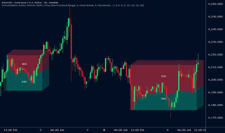
SMT (ICT Concepts)Overview
Smart Money Technique (SMT) Divergence is a price action analysis method derived from Inner Circle Trader (ICT) methodology. This indicator automatically detects SMT divergences by comparing price movements across correlated financial instruments, identifying moments when assets that typically move together begin to diverge - a phenomenon often associated with potential price reversals.
An SMT divergence occurs when one instrument makes a new swing high or low while a correlated instrument fails to confirm that move. This failure to confirm suggests that the instrument may be positioning for a reversal, as the divergence indicates a lack of conviction in the current price direction across related markets.
Theoretical Foundation
What is SMT Divergence?
In correlated markets, instruments tend to move in tandem. For example, the E-mini S&P 500 (ES) and E-mini Nasdaq 100 (NQ) futures typically make swing highs and lows together due to their shared exposure to U.S. equity markets. When this correlation breaks down at key swing points, it creates an SMT divergence.
Bullish SMT Divergence:
The chart instrument creates a lower low compared to a previous swing low, while the correlated comparison instrument creates a higher low (or fails to make a lower low). This divergence at the lows suggests potential buying pressure and a possible bullish reversal.
Bearish SMT Divergence:
The chart instrument creates a higher high compared to a previous swing high, while the correlated comparison instrument creates a lower high (or fails to make a higher high). This divergence at the highs suggests potential selling pressure and a possible bearish reversal.
Why SMT Divergences Matter
SMT divergences are considered significant because they may indicate:
Accumulation or distribution occurring in one instrument but not the other
Relative strength or weakness between correlated assets
Potential exhaustion of the current trend
Early warning signs before major reversals
Indicator Features
Multi-Timeframe SMT Detection
This indicator provides simultaneous SMT detection on two timeframes:
Current Timeframe (CTF) Detection:
The indicator scans for SMT divergences on the chart's active timeframe using multiple pivot lookback periods (3, 5, 8, 13, 21, and 34 bars). This multi-period approach ensures detection of both short-term and intermediate swing points, reducing the likelihood of missing valid divergences while filtering out noise.
Higher Timeframe (HTF) Detection:
Simultaneously, the indicator monitors a higher timeframe for SMT divergences using pivot periods of 3, 5, 8, 13, and 21 HTF candles. Higher timeframe signals generally carry more significance as they represent larger market structure.
Automatic Timeframe Pairing:
When enabled, the indicator automatically selects an appropriate higher timeframe based on your chart's current timeframe:
Sub-1 minute charts pair with 5-minute
1-2 minute charts pair with 15-minute
3-4 minute charts pair with 30-minute
5 minute charts pair with 1-hour
6-9 minute charts pair with 1-hour
15 minute charts pair with 4-hour
16-59 minute charts pair with Daily
1-4 hour charts pair with Weekly
Daily charts pair with Monthly
Combined Signal Detection:
When an SMT divergence is detected on both the current timeframe and higher timeframe at the same price pivots, the indicator combines these into a single enhanced signal. Combined signals display both timeframes in the label and use the higher timeframe styling to emphasize their increased significance.
Automatic Symbol Correlation
The indicator includes comprehensive automatic symbol selection based on the instrument you are viewing. When Auto SMT is enabled, the indicator intelligently selects correlated comparison symbols.
Index Futures Correlations:
E-mini Contracts:
NQ (Nasdaq 100) compares with ES (S&P 500) and YM (Dow Jones)
ES (S&P 500) compares with NQ (Nasdaq 100) and YM (Dow Jones)
YM (Dow Jones) compares with NQ (Nasdaq 100) and ES (S&P 500)
RTY (Russell 2000) compares with ES (S&P 500) and NQ (Nasdaq 100)
Micro Contracts:
MNQ (Micro Nasdaq) compares with MES (Micro S&P) and MYM (Micro Dow)
MES (Micro S&P) compares with MNQ (Micro Nasdaq) and MYM (Micro Dow)
MYM (Micro Dow) compares with MNQ (Micro Nasdaq) and MES (Micro S&P)
M2K (Micro Russell) compares with MES (Micro S&P) and MNQ (Micro Nasdaq)
Metals Futures Correlations:
Standard Contracts:
GC (Gold) compares with SI (Silver) and PL (Platinum)
SI (Silver) compares with GC (Gold) and PL (Platinum)
PL (Platinum) compares with GC (Gold) and SI (Silver)
Micro Contracts:
MGC (Micro Gold) compares with SIL (Micro Silver) and PL (Platinum)
SIL (Micro Silver) compares with MGC (Micro Gold) and PL (Platinum)
Energy Futures Correlations:
CL (Crude Oil) compares with RB (RBOB Gasoline) and NG (Natural Gas)
RB (RBOB Gasoline) compares with CL (Crude Oil) and NG (Natural Gas)
NG (Natural Gas) compares with CL (Crude Oil) and RB (RBOB Gasoline)
MCL (Micro Crude) compares with RB (RBOB Gasoline) and NG (Natural Gas)
Major ETF Correlations:
SPY (S&P 500 ETF) compares with QQQ, DIA, and IWM
QQQ (Nasdaq 100 ETF) compares with SPY, DIA, and IWM
DIA (Dow Jones ETF) compares with SPY, QQQ, and IWM
IWM (Russell 2000 ETF) compares with SPY, QQQ, and DIA
Stock Sector Mapping:
When viewing individual stocks, the indicator automatically identifies the stock's sector and selects appropriate sector ETFs for comparison:
Technology Sector (AAPL, MSFT, GOOGL, NVDA, AMD, INTC, etc.):
Primary: QQQ (Nasdaq 100 ETF)
Secondary: XLK (Technology Select Sector SPDR)
Tertiary: SPY (S&P 500 ETF)
Financial Sector (JPM, BAC, GS, MS, WFC, etc.):
Primary: XLF (Financial Select Sector SPDR)
Secondary: KBE (SPDR S&P Bank ETF)
Tertiary: SPY (S&P 500 ETF)
Energy Sector (XOM, CVX, COP, SLB, etc.):
Primary: XLE (Energy Select Sector SPDR)
Secondary: USO (United States Oil Fund)
Tertiary: SPY (S&P 500 ETF)
Healthcare Sector (JNJ, UNH, PFE, MRK, LLY, etc.):
Primary: XLV (Health Care Select Sector SPDR)
Secondary: IBB (iShares Biotechnology ETF)
Tertiary: SPY (S&P 500 ETF)
Consumer Discretionary Sector (TSLA, HD, NKE, MCD, etc.):
Primary: XLY (Consumer Discretionary Select Sector SPDR)
Secondary: SPY (S&P 500 ETF)
Tertiary: QQQ (Nasdaq 100 ETF)
Consumer Staples Sector (PG, KO, PEP, WMT, COST, etc.):
Primary: XLP (Consumer Staples Select Sector SPDR)
Secondary: SPY (S&P 500 ETF)
Tertiary: QQQ (Nasdaq 100 ETF)
Industrial Sector (CAT, BA, HON, UPS, etc.):
Primary: XLI (Industrial Select Sector SPDR)
Secondary: SPY (S&P 500 ETF)
Tertiary: QQQ (Nasdaq 100 ETF)
Materials Sector (LIN, APD, SHW, FCX, NEM, etc.):
Primary: XLB (Materials Select Sector SPDR)
Secondary: GLD (SPDR Gold Shares)
Tertiary: SPY (S&P 500 ETF)
Utilities Sector (NEE, DUK, SO, etc.):
Primary: XLU (Utilities Select Sector SPDR)
Secondary: SPY (S&P 500 ETF)
Tertiary: QQQ (Nasdaq 100 ETF)
Real Estate Sector (AMT, PLD, CCI, etc.):
Primary: XLRE (Real Estate Select Sector SPDR)
Secondary: VNQ (Vanguard Real Estate ETF)
Tertiary: SPY (S&P 500 ETF)
Communication Services Sector (NFLX, DIS, CMCSA, VZ, T, etc.):
Primary: XLC (Communication Services Select Sector SPDR)
Secondary: SPY (S&P 500 ETF)
Tertiary: QQQ (Nasdaq 100 ETF)
Forex Correlations:
EURUSD compares with GBPUSD
GBPUSD compares with EURUSD
Cryptocurrency Correlations:
BTCUSD compares with ETHUSD
ETHUSD compares with BTCUSD
Three-Symbol Comparison
The indicator supports comparison against up to three symbols simultaneously. When multiple comparison symbols show divergence at the same pivot point, all diverging symbols are displayed in the label, providing stronger confluence. For example, if NQ shows divergence with both ES and YM at the same swing high, the label will display "ES1! + YM1!" indicating divergence confirmation from multiple correlated instruments.
Invalidation Logic
SMT divergences are not indefinitely valid. The indicator includes automatic invalidation logic based on price action following the divergence signal.
Invalidation Rules:
Bearish SMT: Invalidates when price trades above the high of the confirmation pivot (right side of the divergence)
Bullish SMT: Invalidates when price trades below the low of the confirmation pivot (right side of the divergence)
The invalidation level is set at the confirmation bar (the second pivot that completes the SMT pattern), not the extreme of both pivots. This approach aligns with the concept that once price exceeds the confirmation point, the divergence setup is no longer valid.
Invalidation Display Options:
Users can choose to show or hide invalidated SMT signals separately for current timeframe and higher timeframe divergences. When shown, invalidated signals can be displayed with different line styles and widths to visually distinguish them from active signals. Separate limits prevent excessive invalidated signals from cluttering the chart (maximum 15 invalidated signals per timeframe type).
Input Settings
General Settings
Enable SMT Detection:
Master toggle to enable or disable all SMT divergence detection. When disabled, no SMT signals will be calculated or displayed.
Direction:
Filter which divergence types to display:
Both: Display both bullish and bearish SMT divergences
Bullish: Display only bullish SMT divergences (divergence at lows)
Bearish: Display only bearish SMT divergences (divergence at highs)
Symbol Settings
Enable Auto SMT:
When enabled, the indicator automatically selects correlated comparison symbols based on the chart instrument using the correlation mappings described above. When disabled, manual symbol inputs are used.
Symbol 1 (with enable toggle):
First comparison symbol. Enabled by default. When Auto SMT is disabled, enter the desired symbol manually.
Symbol 2 (with enable toggle):
Second comparison symbol. Enabled by default. When Auto SMT is disabled, enter the desired symbol manually.
Symbol 3 (with enable toggle):
Third comparison symbol. Disabled by default. Enable for additional confirmation from a third correlated instrument.
Current Timeframe SMT Settings
Show Current TF SMTs:
Toggle visibility of SMT divergences detected on the chart's current timeframe.
Bullish Color:
Color for bullish SMT divergence lines and labels on the current timeframe.
Bearish Color:
Color for bearish SMT divergence lines and labels on the current timeframe.
Line Style:
Style for current timeframe SMT lines (solid, dashed, or dotted).
Line Width:
Width of current timeframe SMT lines (1-4 pixels).
Show Labels:
Toggle visibility of labels on current timeframe SMT divergences.
Label Style:
Normal: Displays full information including timeframe and diverging symbol names
+/-: Displays minimal "+" or "-" characters with full information available in hover tooltip
Label Size:
Size of current timeframe SMT labels (Tiny, Small, Normal, or Large).
Show Invalidated:
Toggle visibility of invalidated current timeframe SMT signals.
Invalidated Line Style:
Line style for invalidated current timeframe SMT signals.
Invalidated Line Width:
Line width for invalidated current timeframe SMT signals.
Higher Timeframe SMT Settings
Show Higher TF SMTs:
Toggle visibility of SMT divergences detected on the higher timeframe.
Auto Timeframe:
When enabled, automatically selects an appropriate higher timeframe based on the chart's current timeframe. When disabled, uses the manually specified timeframe.
Manual Timeframe:
When Auto Timeframe is disabled, specify the higher timeframe to scan for SMT divergences.
Bullish Color:
Color for bullish SMT divergence lines and labels on the higher timeframe.
Bearish Color:
Color for bearish SMT divergence lines and labels on the higher timeframe.
Line Style:
Style for higher timeframe SMT lines (solid, dashed, or dotted).
Line Width:
Width of higher timeframe SMT lines (1-4 pixels).
Show Labels:
Toggle visibility of labels on higher timeframe SMT divergences.
Label Style:
Normal: Displays full information including timeframe and diverging symbol names
+/-: Displays minimal "+" or "-" characters with full information available in hover tooltip
Label Size:
Size of higher timeframe SMT labels (Tiny, Small, Normal, or Large).
Show Invalidated:
Toggle visibility of invalidated higher timeframe SMT signals.
Invalidated Line Style:
Line style for invalidated higher timeframe SMT signals.
Invalidated Line Width:
Line width for invalidated higher timeframe SMT signals.
Visual Representation
Line Display
SMT divergences are displayed as lines connecting the two pivot points that form the divergence:
For bearish SMT: A line connects the previous swing high to the current (higher) swing high
For bullish SMT: A line connects the previous swing low to the current (lower) swing low
The line color indicates the divergence type (bullish or bearish) and whether it was detected on the current timeframe or higher timeframe.
Label Display
Labels are positioned at the midpoint of the SMT line and display:
The timeframe on which the divergence was detected
The symbol(s) that showed divergence with the chart instrument
When using the "+/-" label style, labels show only "+" for bullish or "-" for bearish divergences, with full information accessible via hover tooltip.
All labels use monospace font formatting for consistent visual appearance.
Combined Signals
When the same divergence is detected on both current and higher timeframes, the signals are combined into a single display using higher timeframe styling. The label shows both timeframes (e.g., "M2 + M15") and all diverging symbols, indicating strong multi-timeframe confluence.
Practical Application Guidelines
Signal Interpretation
SMT divergences should be interpreted within the broader market context. Consider the following when evaluating signals:
Market Structure: SMT divergences occurring at key structural levels (previous highs/lows, order blocks, fair value gaps) tend to be more significant.
Timeframe Confluence: Signals appearing on multiple timeframes simultaneously suggest stronger institutional involvement.
Symbol Confluence: Divergences confirmed by multiple comparison symbols indicate broader market disagreement with the current price direction.
Time of Day: SMT divergences during high-volume trading sessions may carry more weight than those during low-liquidity periods.
Limitations and Considerations
Correlation Variability: Correlations between instruments can strengthen or weaken over time. The automatic symbol selection is based on typical correlations but may not always reflect current market conditions.
Pivot Detection Lag: Pivots are only confirmed after subsequent price action, meaning SMT signals appear with some delay after the actual swing point forms.
False Signals: Not all SMT divergences result in reversals. Use additional confirmation methods and proper risk management.
Data Requirements: The indicator requires sufficient historical data and may not function properly on instruments with limited price history.
Technical Notes
The indicator uses multiple pivot detection periods to identify swing points across different scales
Higher timeframe candle tracking is performed on the lower timeframe chart for precise pivot bar indexing
A deduplication system prevents the same divergence from being detected multiple times across different pivot periods
Array-based storage manages active and invalidated SMT signals with automatic cleanup to prevent memory issues
Maximum label and line counts are set to 500 each to accommodate extended analysis periods
Disclaimer
This indicator is provided for educational and informational purposes only. It is designed to assist traders in identifying potential SMT divergences based on historical price data and should not be considered as financial advice or a recommendation to buy or sell any financial instrument.
Trading financial markets involves substantial risk of loss and is not suitable for all investors. Past performance of any trading methodology, including concepts discussed in this indicator, does not guarantee future results. Users should conduct their own research and analysis before making any trading decisions.
The automatic symbol correlations and sector mappings are based on general market relationships and may not accurately reflect current or future correlations. Users are encouraged to verify correlations independently and adjust comparison symbols as needed.
Always use appropriate risk management techniques, including but not limited to position sizing and stop-loss orders. Never risk more capital than you can afford to lose.

SMC Pro+ ICT v4 Enhanced - FINAL🎯 SMC Pro+ ICT v4 Enhanced - Complete Smart Money Trading System📊 Professional All-in-One Indicator for Smart Money Concepts & ICT MethodologyThe SMC Pro+ ICT v4 Enhanced is a comprehensive trading system that combines Smart Money Concepts (SMC) with Inner Circle Trader (ICT) methodology. This indicator provides institutional-grade market structure analysis, liquidity mapping, and volume profiling in one powerful package.✨ CORE FEATURES🏗️ Advanced Market Structure Detection
MSS (Market Structure Shift) - Identifies major trend reversals with precision
BOS (Break of Structure) - Confirms trend continuation moves
CHoCH (Change of Character) - Detects internal structure shifts
Modern LuxAlgo-Style Lines - Clean, professional visualization
Dual Sensitivity System - External structure (major swings) + Internal structure (minor swings)
Customizable Labels - Tiny, Small, or Normal sizes
Structure Break Visualization - Clear break point markers
💎 Supply & Demand Zones (POI - Point of Interest)
Institutional Order Blocks - Where smart money enters/exits
ATR-Based Zone Sizing - Dynamically adjusted to market volatility
Smart Overlap Detection - Prevents cluttered charts
Historical Zone Tracking - Maintains up to 50 zones
POI Central Lines - Pinpoint entry/exit levels
Auto-Extension - Zones extend to current price
Auto-Cleanup - Removes broken zones automatically
📦 Fair Value Gap (FVG) Detection
Bullish & Bearish FVGs - Institutional inefficiencies
Consequent Encroachment (CE) - 50% fill levels
Auto-Delete Filled Gaps - Keeps charts clean
Customizable Lookback - 1-30 days of history
Color-Coded Zones - Easy visual identification
CE Line Styles - Dotted, Dashed, or Solid
🚀 Enhanced PVSRA Volume Analysis
This is one of the most powerful features:
200% Volume Candles - Extreme institutional activity (Lime/Red)
150% Volume Candles - High institutional interest (Blue/Fuchsia)
Volume Climax Detection - Major reversal signals with 2.5x+ volume
Exhaustion Signals - Identifies buying/selling exhaustion with high accuracy
Enhanced Volume Divergence - NEW! High-quality reversal detection
Price makes lower low, Volume makes higher low = Bullish Divergence
Price makes higher high, Volume makes lower high = Bearish Divergence
Strict trend context filtering for accuracy
Rising/Falling Volume Patterns - Momentum confirmation (allows 1 exception in 3 bars)
Volume Spread Analysis - Price range × Volume for true strength
Body/Wick Ratio Analysis - Candle structure quality
ATR Normalization - Adjusts for different market volatility
Volume Profile Indicators - 🔥 EXTREME, ⚡ VERY HIGH, 📈 HIGH, ✅ ABOVE AVG
💧 Advanced Liquidity System
Smart money targets these levels:
Weekly High/Low Liquidity - Major institutional targets
Daily High/Low Liquidity - Intraday key levels
4H Session Liquidity - Short-term targets
Distance Indicators - Shows % distance from current price
Strength Indicators - Identifies high-probability sweeps
Swept Level Detection - Tracks executed liquidity grabs
Customizable Line Styles - Width, length, offset controls
Color-Coded Levels - Easy visual hierarchy
🎯 Master Bias System
Data-driven directional bias with 9-factor scoring:
Bull/Bear Bias Calculation - 0-100% scoring system
Multi-Timeframe Analysis - Daily, 4H, 1H trend alignment
Kill Zone Integration - London (2-5 AM) & NY (8-11 AM) sessions
EMA Alignment Factor - Trend confirmation
Volume Confirmation - Adds 5% when volume supports direction
Range Filter Integration - Adds 10% for trending markets
Session Context - Above/below session midpoint scoring
Bias Strength Rating - STRONG (>75%), MODERATE (60-75%), WEAK (<60%)
Real-Time Updates - Dynamic recalculation
📈 Premium & Discount Zones
Fibonacci-based institutional pricing:
Extreme Premium - Above 78.6% (Overvalued)
Premium Zone - 61.8% - 78.6% (Expensive)
Equilibrium - 38.2% - 61.8% (Fair Value)
Discount Zone - 21.4% - 38.2% (Cheap)
Extreme Discount - Below 21.4% (Undervalued)
Visual Zone Boxes - Color-coded for instant recognition
200-500 Bar Lookback - Customizable range calculation
🔄 Range Filter
Advanced trend detection:
Smoothed Range Calculation - Eliminates noise
Dynamic Support/Resistance - Auto-adjusting levels
Upward/Downward Counters - Measures trend strength
Color-Coded Line - Green (uptrend), Red (downtrend), Orange (ranging)
Adjustable Period - 1-200 bars
Multiplier Control - Fine-tune sensitivity (0.1-10.0)
🌊 Liquidity Zones (Vector Zones)
PVSRA-based horizontal liquidity:
Above Price Zones - Resistance clusters
Below Price Zones - Support clusters
Maximum 500 Zones - Professional-grade capacity
Body/Wick Definition - Choose zone boundaries
Auto-Cleanup - Removes cleared zones
Color Override - Custom styling options
Transparency Control - 0-100% opacity
📊 EMA System
Triple EMA trend confirmation:
Fast EMA (9) - Green line - Immediate trend
Medium EMA (21) - Blue line - Short-term trend
Slow EMA (50) - Red line - Major trend
EMA Alignment Detection - Bull/Bear stack confirmation
Dashboard Integration - Status: 📈 BULL ALIGN, 📉 BEAR ALIGN, 🔀 MIXED
Adjustable Lengths - Customize all three EMAs (5-200)
🎯 IDM (Institutional Decision Maker) Levels
Key institutional price levels:
Latest IDM Detection - 20-bar pivot lookback
Extended Lines - Projects 50 bars into future
Customizable Styles - Solid, Dashed, or Dotted
Line Width Control - 1-5 pixels
Color Selection - Match your chart theme
Price Label - Shows exact level with tick precision
📱 Professional Dashboard
Real-time market intelligence panel:
🎯 SIGNAL - 🟢 LONG, 🔴 SHORT, ⏳ WAIT, 🛑 NO TRADE
🎲 BIAS - Bull/Bear with STRONG/MODERATE/WEAK rating
📊 BULL/BEAR Scores - 0-100% percentage display
💎 ZONE - Current premium/discount location
🕐 KZ - Kill Zone status (🇬🇧 LONDON/🇺🇸 NY/⏸️ OFF)
🏗️ STRUCT - Market structure status (BULLISH/BEARISH/NEUTRAL)
⚡ EVENT - Last structure event (MSS/BOS)
⚡ INT - Internal structure trend
🎯 IDM - Latest institutional level
📊 EMA - EMA alignment status
🔄 RF - Range Filter direction
📊 PVSRA - Volume status (🚀 CLIMAX/📈 RISING/📉 FALLING)
📅 MTF - Multi-timeframe alignment (✅ FULL/⚠️ PARTIAL/❌ CONFLICT)
💪 CONF - Confidence score (0-100%)
📊 VOL - Volume ratio (e.g., 1.8x average)
Advanced Metrics (Toggle On/Off):
📏 RSI - Value + Status (OVERBOUGHT/STRONG/NEUTRAL/WEAK/OVERSOLD)
📈 MACD - Value + Direction (BULL/BEAR)
🌪️ VOL - Volatility state (⚠️ EXTREME/🔥 HIGH/📊 NORMAL/😴 LOW)
🔊 VOL PROF - Volume profile ratio
⏱️ TF - Current timeframe
Dashboard Customization:
4 Positions - Top Left, Top Right, Bottom Left, Bottom Right
3 Sizes - Small, Normal, Large
2 Modes - Compact (MTF combined) or Full (separate rows)
Professional Design - Dark theme with color-coded cells
🎮 TRADING SIGNALS & SETUP SCORING🟢 LONG Setup Requirements (9-Factor Confidence Score)
MTF Alignment - Daily/4H/1H/Structure all bullish (+2 points for full, +1 for partial)
Volume Confirmation - Above 1.2x average (+1 point)
Structure Event - MSS or BOS bullish (+2 points)
EMA Alignment - 9 > 21 > 50 (+1 point)
Kill Zone Active - London/NY + Bull bias >75% (+2 points)
Bias Match - Master bias matches structure trend (+1 point)
Confidence Threshold - >60% minimum for signal
🔴 SHORT Setup Requirements
Same 9-factor system but inverted for bearish conditions.💪 Confidence Levels
75-100% - ⭐ HIGH CONFIDENCE (Strong setup, all factors aligned)
50-74% - ⚠️ MODERATE (Good setup, partial alignment)
0-49% - ❌ LOW CONFIDENCE (Wait for better setup)
🎯 Signal Output
🟢 LONG - Bull bias + Bullish structure + >60% confidence
🔴 SHORT - Bear bias + Bearish structure + >60% confidence
⏳ WAIT LONG - Bull bias but low confidence
⏳ WAIT SHORT - Bear bias but low confidence
🛑 NO TRADE - Neutral bias or conflicting signals
🔔 COMPREHENSIVE ALERT SYSTEM (12 Alerts)Structure Alerts
⚡ MSS Bullish - Major bullish reversal
⚡ MSS Bearish - Major bearish reversal
📈 BOS Bullish - Bullish continuation
📉 BOS Bearish - Bearish continuation
⚠️ CHoCH Bullish - Internal bullish shift
⚠️ CHoCH Bearish - Internal bearish shift
Bias & Confidence Alerts
🟢 Bias Shift Bull - Master bias turns bullish
🔴 Bias Shift Bear - Master bias turns bearish
⭐ High Confidence - Setup reaches 75%+ confidence
Volume Alerts (High Probability)
🚀 Volume Climax Buy - Extreme bullish volume spike
💥 Volume Climax Sell - Extreme bearish volume spike
⚠️ Selling Exhaustion - Potential bullish reversal
⚠️ Buying Exhaustion - Potential bearish reversal
📊 Bullish Volume Divergence - High-quality bullish reversal signal
📊 Bearish Volume Divergence - High-quality bearish reversal signal
🎨 EXTENSIVE CUSTOMIZATIONColors & Styling
✅ All colors customizable for every component
✅ Supply/Demand zone colors + outlines
✅ FVG colors (bullish/bearish)
✅ PVSRA candle colors (6 types)
✅ Liquidity level colors (Weekly/Daily/4H/Swept)
✅ Structure line colors
✅ Premium/Equilibrium/Discount zone colorsDisplay Controls
✅ Toggle each feature on/off independently
✅ Adjustable sensitivities (Structure: 5-30, Internal: 3-15)
✅ Label size controls (Tiny/Small/Normal)
✅ Line width adjustments (1-5 pixels)
✅ Transparency controls (0-100%)
✅ Extension lengths (20-100 bars)
✅ Lookback periods (50-500 bars)Volume Settings
✅ PVSRA symbol override (trade one asset, analyze another)
✅ Climax threshold (2.0-5.0x)
✅ Rising volume bar count (2-5 bars)
✅ Divergence filters (Strict/Lenient)
✅ Divergence minimum bars (10-30)
✅ Volume threshold multiplier (1.0-2.0x)Dashboard Settings
✅ Position (4 corners)
✅ Size (Small/Normal/Large)
✅ Compact/Full mode
✅ Show/Hide advanced metrics
✅ Show/Hide EMA status💡 BEST PRACTICES & USAGE TIPS⏰ Optimal Timeframes
Scalping - 1m, 5m (Use Kill Zones, Volume Climax, FVG)
Day Trading - 5m, 15m, 1H (Use Structure, Liquidity, Bias)
Swing Trading - 4H, Daily (Use MTF, Premium/Discount, Structure)
Position Trading - Daily, Weekly (Use major structure, liquidity)
🎯 Asset Classes
✅ Forex - All pairs (especially majors during Kill Zones)
✅ Crypto - BTC, ETH, altcoins (24/7 liquidity)
✅ Stocks - All stocks and indices (use session times)
✅ Commodities - Gold, Silver, Oil (high volume periods)
✅ Indices - S&P 500, NASDAQ, DAX, etc.🔥 High-Probability Setups
The Perfect Storm
MSS in direction of daily trend
Kill Zone active
Volume climax
Confidence >75%
Price in discount (long) or premium (short)
Volume Divergence Play
Enhanced volume divergence signal
CHoCH confirms direction change
Price near liquidity level
FVG forms for entry
Liquidity Sweep
Price sweeps weekly/daily high/low
Immediate rejection (selling/buying exhaustion)
Structure shift (MSS)
Volume confirmation
Structure Retest
BOS breaks structure
Price returns to POI/FVG
Volume confirms (>1.2x)
Kill Zone active
📊 Multi-Timeframe Analysis
Higher Timeframe - Identify trend & structure (Daily/4H)
Trading Timeframe - Find entries (15m/1H)
Lower Timeframe - Precise entries (1m/5m)
Look for MTF alignment - Dashboard shows ✅ FULL or ⚠️ PARTIAL
⚠️ Risk Management
Always use stop-loss (below/above recent structure)
Position size: 1-2% risk per trade
Target liquidity levels for take profit
Use supply/demand zones for SL placement
Watch for exhaustion signals near targets

First FVG After 9:30 AM ET + Opening Range (1min) OK# FVG + Opening Range Breakout Indicator (1M)
## Overview
A professional trading indicator designed for 1-minute candlestick charts that identifies Fair Value Gaps (FVG) and Opening Range breakout patterns with precise entry signals for institutional trading strategies.
## Key Features
### 1. Fair Value Gap Detection (FVG)
- **Automatic Detection**: Identifies the first FVG after 9:30 AM ET
- **Support for Both Types**:
- **Bearish FVG**: Gap formed when candle 3 high is below candle 1 low (downward gap)
- **Bullish FVG**: Gap formed when candle 3 low is above candle 1 high (upward gap)
- **Visual Representation**: Blue box marking the exact gap zone
- **Active Period**: 9:30 AM - 2:00 PM ET only
### 2. FVG Entry Signals
- **SELL Signal (Bearish FVG)**: Generated when price enters and respects the gap
- Triggers when close stays within the FVG range
- Multiple signals allowed on retests
- Position label placed above bearish candles
- **BUY Signal (Bullish FVG)**: Generated when price breaks above FVG top
- Triggers when close breaks above fvgHigh
- Allows multiple signals on subsequent retests
- Position label placed below bullish candles
### 3. Opening Range (9:30 - 10:00 AM ET)
- **Three Key Levels**:
- **OR High** (Red Dashed Line): Highest point during opening 30 minutes
- **OR Low** (Green Dashed Line): Lowest point during opening 30 minutes
- **OR Mid** (Orange Dotted Line): Midpoint between High and Low
- **Lines Extend**: 100 bars into the session for reference
### 4. Opening Range Breakout Signals
Detects breakouts from the opening range with a refined entry strategy:
- **BUY Signal (OR High Breakout)**:
1. Price breaks ABOVE OR High (high1m > orHigh)
2. Waits minimum 5 candles
3. Price retests OR High level (close ≤ orHigh)
4. Price rebounds UPWARD (close > orHigh)
5. Signal generated with label "BUY"
- **SELL Signal (OR Low Breakout)**:
1. Price breaks BELOW OR Low (low1m < orLow)
2. Waits minimum 5 candles
3. Price retests OR Low level (close ≥ orLow)
4. Price rebounds DOWNWARD (close < orLow)
5. Signal generated with label "SELL"
### 5. Time Filters
- **Session Start**: 9:30 AM ET (Market Open)
- **Session End**: 2:00 PM ET (14:00)
- **All signals only generated within this window**
- **Daily Reset**: All data clears at market open each trading day
## Settings
| Parameter | Default | Description |
|-----------|---------|-------------|
| FVG Box Color | Blue (80% transparent) | Visual color of FVG zone |
| FVG Border Color | Blue | Border line color |
| Border Width | 1 | Thickness of FVG box border |
| Box Extension Right | 20 bars | How far right the box extends |
| Box Extension Left | 5 bars | How far left the box extends |
| Minimum FVG Size | 5.0 points | Minimum gap size to display |
| FVG Respect Tolerance | 2.0 points | Price tolerance for FVG respect |
| Show FVG Labels | True | Display "First FVG" label |
| Show Signals | True | Display SELL/BUY entry signals |
| Show Opening Range | True | Display OR High/Low/Mid lines |
| OR High Color | Red (80% transparent) | OR High line color |
| OR Low Color | Green (80% transparent) | OR Low line color |
| OR Mid Color | Orange (80% transparent) | OR Mid line color |
| OR Line Width | 2 | Thickness of OR lines |
| OR Line Length | 100 bars | Extension of OR lines |
| Timezone Offset | -5 (EST) | UTC offset (-4 for EDT) |
## Trading Strategy Integration
### Institutional Trading Approach
This indicator combines two professional trading methodologies:
1. **Fair Value Gap Trading**: Exploits market inefficiencies (gaps) that institutional traders fill during the day
2. **Opening Range Breakout**: Captures momentum moves that break out of the morning consolidation
### Optimal Use Cases
- **Asian Session into London Open**: Monitor FVG formation
- **Pre-Market Gap Analysis**: Plan breakout trades
- **Early Morning Momentum**: Catch OR breakouts with precision entries
- **Intraday Scalping**: Use signals for quick risk/reward entries
### Risk Management
- Entry signals clearly marked with labels
- Trailing stops can be set at OR levels
- Multiple timeframe confirmation recommended
- Always use stop losses below/above key levels
## Signal Interpretation
| Signal | Type | Action | Location |
|--------|------|--------|----------|
| SELL | FVG Bearish | Short Entry | Above bearish candle |
| BUY | FVG Bullish | Long Entry | Below bullish candle |
| BUY | OR High Breakout | Long Entry | Above OR High |
| SELL | OR Low Breakout | Short Entry | Below OR Low |
## Color Scheme
- **Red**: Bearish direction (SELL signals, OR High)
- **Green**: Bullish direction (BUY signals, OR Low)
- **Orange**: Neutral reference (OR Mid point)
- **Blue**: FVG zones (gaps)
- **Yellow**: Background during FVG search phase
## Notes
- Indicator works exclusively on 1-minute charts
- Requires market open data (9:30 AM ET)
- All times referenced to Eastern Time (ET)
- Historical data should include full trading day for accuracy
- Use with volume and momentum indicators for confirmation
---
**Designed for professional traders using institutional-grade trading methodologies**

ACCDv3# ACCDv3 - Accumulation/Distribution MACD with Divergence Detection
## Overview
**ACCDv3** (Accumulation/Distribution MACD Version 3) is an advanced volume-weighted momentum indicator that combines the Accumulation/Distribution (A/D) line with MACD methodology and divergence detection. It helps identify trend strength, momentum shifts, and potential reversals by analyzing volume-weighted price movements.
## Key Features
- **Volume-Weighted MACD**: Applies MACD calculation to volume-weighted A/D values for earlier, more reliable signals
- **Divergence Detection**: Identifies when A/D trend diverges from MACD momentum
- **Volume Strength Filtering**: Distinguishes high-volume confirmations from low-volume noise
- **Color-Coded Histogram**: 4-color system showing momentum direction and volume strength
- **Real-Time Alerts**: Background colors and alert conditions for bullish/bearish divergences
## Components
### 1. Accumulation/Distribution (A/D) Line
The A/D line measures buying and selling pressure by comparing the close price to the trading range, weighted by volume:
```
A/D = Σ ((2 × Close - Low - High) / (High - Low)) × Volume
```
- **Rising A/D**: More accumulation (buying pressure)
- **Falling A/D**: More distribution (selling pressure)
- **Doji Handling**: When High = Low, contribution is zero (avoids division errors)
### 2. Volume-Weighted MACD
Instead of simple EMAs, the indicator weights A/D values by volume:
- **Fast Line** (default 12): `EMA(A/D × Volume, 12) / EMA(Volume, 12)`
- **Slow Line** (default 26): `EMA(A/D × Volume, 26) / EMA(Volume, 26)`
- **MACD Line**: Fast Line - Slow Line (green line)
- **Signal Line** (default 9): EMA or SMA of MACD (orange line)
- **Histogram**: MACD - Signal (color-coded columns)
This volume-weighting ensures that periods with higher volume have greater influence on the indicator values.
### 3. Histogram Color System
The histogram uses 4 distinct colors based on **direction** and **volume strength**:
| Condition | Color | Meaning |
|-----------|-------|---------|
| Rising + High Volume | **Dark Green** (#1B5E20) | Strong bullish momentum with volume confirmation |
| Rising + Low Volume | **Light Teal** (#26A69A) | Bullish momentum but weak volume (less reliable) |
| Falling + High Volume | **Dark Red** (#B71C1C) | Strong bearish momentum with volume confirmation |
| Falling + Low Volume | **Light Red/Pink** (#FFCDD2) | Bearish momentum but weak volume (less reliable) |
Additional shading:
- **Light Cyan** (#B2DFDB): Positive but not rising (momentum stalling)
- **Bright Red** (#FF5252): Negative and accelerating down
### 4. Divergence Detection
Divergence occurs when A/D trend and MACD momentum move in opposite directions:
#### Bullish Divergence (Green Background)
- **Condition**: A/D is trending up BUT MACD is negative and trending down
- **Interpretation**: Accumulation increasing while momentum appears weak
- **Signal**: Potential bullish reversal or continuation
- **Action**: Look for entry opportunities or hold long positions
#### Bearish Divergence (Red Background)
- **Condition**: A/D is trending down BUT MACD is positive and trending up
- **Interpretation**: Distribution increasing while momentum appears strong
- **Signal**: Potential bearish reversal or weakening uptrend
- **Action**: Consider exits, tighten stops, or prepare for reversal
## Parameters
| Parameter | Default | Range | Description |
|-----------|---------|-------|-------------|
| **Fast Length** | 12 | 1-50 | Period for fast EMA (shorter = more sensitive) |
| **Slow Length** | 26 | 1-100 | Period for slow EMA (longer = smoother) |
| **Signal Smoothing** | 9 | 1-50 | Period for signal line (MACD smoothing) |
| **Signal Line MA Type** | EMA | SMA/EMA | Moving average type for signal calculation |
| **Volume MA Length** | 20 | 5-100 | Period for volume average (strength filter) |
## Usage Guide
### Reading the Indicator
1. **MACD Lines (Green & Orange)**
- **Crossovers**: When green crosses above orange = bullish, below = bearish
- **Distance**: Wider gap = stronger momentum
- **Zero Line**: Above = bullish bias, below = bearish bias
2. **Histogram Colors**
- Focus on **dark colors** (dark green/red) for high-confidence signals
- Be cautious with **light colors** (teal/pink) - wait for volume confirmation
- Watch for **rising red bars** (V-bottom pattern) = potential bullish reversal
- Watch for **falling green bars** (Λ-top pattern) = potential bearish reversal
3. **Background Divergence Alerts**
- **Green background**: Bullish divergence - consider long entries
- **Red background**: Bearish divergence - consider exits or shorts
- Best used in combination with price action and support/resistance levels
### Trading Strategies
#### Trend Following
1. Wait for MACD to cross above zero line with dark green histogram
2. Enter long when histogram shows consecutive dark green bars
3. Exit when histogram turns light green or red appears
#### Divergence Trading
1. Wait for background divergence alert (green or red)
2. Confirm with price action (support/resistance, candlestick patterns)
3. Enter on next dark-colored histogram bar in divergence direction
4. Set stops beyond recent swing high/low
#### Volume Confirmation
1. Ignore signals during low-volume periods (light colors)
2. Take aggressive positions during high-volume confirmations (dark colors)
3. Use volume strength as position sizing guide (larger size on dark bars)
### Best Practices
✓ **Combine with price action**: Don't rely on indicator alone
✓ **Wait for dark colors**: High-volume bars are more reliable
✓ **Watch for divergences**: Early warning signs of reversals
✓ **Use multiple timeframes**: Confirm signals across 1m, 5m, 15m
✓ **Respect zero line**: Trading direction should align with MACD side
✗ **Don't chase light-colored signals**: Low volume = lower reliability
✗ **Don't ignore context**: Market structure and levels matter
✗ **Don't over-trade**: Wait for clear, high-volume setups
✗ **Don't ignore alerts**: Divergences are early warnings
## Technical Details
### Volume-Weighted Calculation Method
Traditional MACD uses simple price EMAs. ACCDv3 weights each A/D value by its corresponding volume:
```pine
// Volume-weighted fast EMA
close_vol_fast = ta.ema(ad × volume, fast_length)
vol_fast = ta.ema(volume, fast_length)
vw_ad_fast = close_vol_fast / vol_fast
// Same for slow EMA
close_vol_slow = ta.ema(ad × volume, slow_length)
vol_slow = ta.ema(volume, slow_length)
vw_ad_slow = close_vol_slow / vol_slow
// MACD is the difference
macd = vw_ad_fast - vw_ad_slow
```
This ensures high-volume periods have proportionally more impact on the indicator.
### Volume Strength Filter
Determines whether current volume is above or below average:
```pine
vol_avg = ta.sma(volume, vol_length)
vol_strength = volume > vol_avg
```
Used to select dark (high volume) vs light (low volume) histogram colors.
### Divergence Logic
```pine
// A/D trending up if above its 5-period SMA
ad_trend = ad > ta.sma(ad, 5)
// MACD trending up if above zero
macd_trend = macd > 0
// Divergence when trends oppose
divergence = ad_trend != macd_trend
// Specific conditions
bullish_divergence = ad_trend and not macd_trend and macd < 0
bearish_divergence = not ad_trend and macd_trend and macd > 0
```
## Alerts
The indicator includes built-in alert conditions:
- **Bullish Divergence**: "Bullish Divergence: A/D trending up but MACD trending down"
- **Bearish Divergence**: "Bearish Divergence: A/D trending down but MACD trending up"
To enable:
1. Click "Create Alert" button in TradingView
2. Select "ACCDv3" as condition
3. Choose "Bullish Divergence" or "Bearish Divergence"
4. Configure notification method (popup, email, webhook, etc.)
## Comparison with Standard MACD
| Feature | Standard MACD | ACCDv3 |
|---------|---------------|---------|
| **Input** | Close price | Accumulation/Distribution line |
| **Weighting** | Simple EMA | Volume-weighted EMA |
| **Divergence** | Price vs MACD | A/D vs MACD |
| **Volume Analysis** | None | Built-in strength filter |
| **Color System** | 2 colors (up/down) | 4+ colors (direction + volume) |
| **Leading/Lagging** | Lagging | More leading (volume-weighted) |
## Example Scenarios
### Scenario 1: Strong Bullish Signal
- **Chart**: MACD crosses above zero line
- **Histogram**: Dark green bars (#1B5E20) appearing
- **Volume**: Above 20-period average
- **Action**: Enter long, strong momentum with volume confirmation
### Scenario 2: Weak Bearish Signal
- **Chart**: MACD crosses below zero line
- **Histogram**: Light pink bars (#FFCDD2) appearing
- **Volume**: Below 20-period average
- **Action**: Avoid shorting, low volume = unreliable signal
### Scenario 3: Bullish Divergence Reversal
- **Chart**: Price making lower lows
- **Indicator**: A/D line trending up, MACD negative
- **Background**: Green shading appears
- **Histogram**: Transitions from red to dark green
- **Action**: Look for long entry on next dark green bar
### Scenario 4: V-Bottom Reversal
- **Chart**: Downtrend in place
- **Histogram**: Red bars start rising (becoming less negative)
- **Pattern**: Forms "V" shape at bottom
- **Confirmation**: Transitions to dark green bars
- **Action**: Bullish reversal signal, consider long entry
## Timeframe Recommendations
- **1-minute**: Scalping, very fast signals (noisy, use with caution)
- **5-minute**: Intraday momentum trading (recommended)
- **15-minute**: Swing entries, clearer trend signals
- **1-hour+**: Position trading, major trend identification
## Limitations
- **Requires volume data**: Will not work on instruments without volume
- **Lag during consolidation**: MACD is inherently trend-following
- **False signals in chop**: Sideways markets generate noise
- **Not a standalone system**: Should be combined with price action and risk management
## Version History
- **v3**: Removed traditional price MACD, using only volume-weighted A/D MACD with A/D divergence
- **v2**: Added A/D divergence detection, volume strength filtering, enhanced histogram colors
- **v1**: Basic MACD on A/D line with volume-weighted calculation
## Support & Further Reading
For questions, updates, or to report issues, refer to the main project documentation or contact the developer.
**Related Indicators in Suite:**
- **VMACDv3**: Volume-weighted MACD on price (not A/D)
- **RSIv2**: RSI with A/D divergence
- **DMI**: Directional Movement Index with A/D divergence
- **Elder Impulse**: Bar coloring system using volume-weighted MACD
---
*This indicator is for educational purposes. Always practice proper risk management and never risk more than you can afford to lose.*

BB/KC Squeeze Channels (v6)Technical Specification for the BB/KC Squeeze Volatility Indicator in Algorithmic Cryptocurrency Trading
I. Theoretical Foundations of Volatility Dynamics
The "Contraction-Expansion" Principle (Volatility Contraction/Expansion)
The fundamental analysis of market volatility dynamics relies on the principle popularized by John Bollinger: periods of low volatility are inevitably followed by periods of high volatility. This phenomenon, known as the cyclical nature of volatility, is the cornerstone of trading strategies based on range breakouts (Breakout Strategy). In the context of technical analysis, volatility contraction manifests as a consolidation phase where the trading range narrows, preceding a strong, directional price impulse.
The essence of volatility contraction lies in a phase of market equilibrium that is inherently unstable. Most often, this reflects the covert activities of large market participants who are either accumulating or distributing a significant volume of the asset. These actions occur within a narrow price corridor to avoid sharp price movements until the entire position is acquired. As a result, activity decreases, the range narrows, and the market accumulates "energy" for the subsequent large-scale expansion. For the cryptocurrency market, characterized by high impulsivity and a tendency toward sharp trending moves, accurately identifying the deep contraction phase becomes a powerful algorithmic predictor.
Identifying Prerequisites: Distinguishing Pre-Breakout Contraction
To build a reliable indicator, it is crucial to distinguish a true pre-breakout squeeze from other types of volatility reduction that do not lead to a strong impulse. Specifically, volatility, measured by the Average True Range (ATR), will always decline after the completion of a strong vertical movement, as the market enters a pullback or deceleration phase. Such a decline is post-impulse and does not necessarily signal an imminent breakout.
It is necessary to find signs of abnormally low volatility that occurs precisely in the consolidation phase. The optimal time to look for a Squeeze signal is the formation of a distinct sideways channel. In this phase, the middle line of the channel indicator (e.g., EMA or SMA) should be relatively horizontal. This confirms that the market is currently in a ranging state (absence of a strong current trend), not in a deceleration phase after a trend. Therefore, the Squeeze indicator algorithm must include a check for confirmed sideways movement (e.g., through analyzing the slope of the middle line or its statistical deviation from the horizontal over the last X periods). Only abnormally low volatility during a range can be classified as a high-confidence pre-breakout contraction.
II. Instrument Selection: Justification for the Composite BB/KC Squeeze Approach
For effective algorithmic determination of the extreme contraction phase, it is necessary to use an indicator that combines the advantages of the two most reliable methods for measuring volatility: Bollinger Bands and Keltner Channels.
Comparative Analysis of Volatility Indicators
| Indicator | Base Metric | Volatility Response | Primary Role in Squeeze |
|---|---|---|---|
| Bollinger Bands (BB) | Standard Deviation (SD) | Fast, Highly Sensitive | Contraction sensor, Early breakout signal |
| Keltner Channels (KC) | Average True Range (ATR) | Smooth, Noise Filtering | Defines stable range, Filters false signals |
Bollinger Bands (BB)
Bollinger Bands are based on the Standard Deviation (SD) of the price from a moving average. This statistical metric makes BB highly sensitive, as they quickly react to sudden changes in volatility. Due to this sensitivity, BB are ideal for early registration of a contraction and for generating the breakout signal. However, their high sensitivity is also a drawback, as it can lead to false signals and premature expansion during market noise.
Keltner Channels (KC)
Keltner Channels, in the modern version developed by Linda Raschke, use the Average True Range (ATR) to calculate the channel width. ATR represents the averaged true range of fluctuations, which provides a smoother and more stable measure of volatility. KC react to market changes slower than BB, but their smoothness allows for better filtering of false signals and determination of the true direction of movement. Unlike fixed-width price channels or percentage envelopes, which perform poorly in dynamic environments, BB and KC automatically adapt to market conditions.
The Squeeze Mechanism: Synergy of Instruments
The BB/KC Squeeze indicator uses the synergy of BB and KC to achieve maximum accuracy in identifying the accumulation phase.
The technical Squeeze condition (Squeeze ON) is defined when the fast and statistically-oriented Bollinger Bands (BB) are inside the wider and smoother Keltner Channels (KC). This state represents quantitative confirmation of extremely low volatility.
In standard settings, BB use a multiplier of 2.0 for Standard Deviation (SD), and KC use a multiplier of 1.5 for ATR. For the statistical width of BB (based on price deviation from the average) to narrow inside the width of KC (based on the averaged range), the current statistical deviation of the price must fall to abnormally low values relative to the historical average range of fluctuations. This is not just low volatility, but its extreme contraction, indicating maximum accumulation of potential energy before an impulse.
III. Quantitative Analysis: How Much, Why, and How Volatility Contracts
How Much: Mathematical Definition of the Degree of Contraction
The degree of volatility contraction before a breakout is measured through a strict mathematical condition that ensures the current volatility is significantly below its averaged historical value.
The Squeeze Condition (Squeeze ON) requires both of the following mathematical formulas to be true :
To understand how much the movement should contract, we must consider the channel width formulas:
* Bollinger Bands Width (\text{BB}_{\text{Width}}):
\text{KC}_{\text{Width}} = 2 \times (\text{ATR} \times 1.5) = 3.0 \times \text{ATR}$$
The Squeeze ON state means that \text{BB}_{\text{Width}} < \text{KC}_{\text{Width}}. This condition is equivalent to \text{SD} \times 4.0 < \text{ATR} \times 3.0. As a result, the current Standard Deviation (SD) must fall below 75% of the Average True Range (ATR) for the contraction to be registered. This requirement for SD to decrease to a level significantly below ATR is the criterion for identifying the deep market calm that serves as the energy base for the subsequent directional movement.
Why and How: Qualitative Signs
Volatility decreases because large market participants are slowly and covertly accumulating positions. They keep the price within a narrow range to fully acquire the necessary volume before allowing the price to impulsively exit consolidation. This creates a sideways movement phase, minimizing risks for the trader and enabling timely tracking of a bullish or bearish breakout.
To enhance the algorithm's reliability and prevent entry into false ranges, the following qualitative signs accompanying a true squeeze must be considered:
* Squeeze Duration: The longer the price remains in the Squeeze ON state, the more energy is accumulated. Experience suggests a minimum duration of 4–8 periods. Extended contraction periods (over 10–12 bars) often precede the strongest impulsive movements in the crypto market.
* Price Position: During the contraction phase, the price should remain close to the middle line (EMA/SMA). This confirms that the market is in equilibrium, and accumulation is occurring around the "fair" price of the current range.
* Momentum Context: The volatility indicator (BB/KC) determines when a move will happen, but not its direction. To predict the direction (prerequisite), a momentum component must be used (e.g., a histogram, as in the TTM Squeeze variant ). The appearance of positive momentum during the contraction, even without price movement, signals potential bullish strength, increasing the likelihood of an upward breakout.
Squeeze State Logic Table
| State | Mathematical Condition (BB vs KC) | Market Interpretation |
|---|---|---|
| Squeeze ON | (\text{BB}_{\text{Upper}} < \text{KC}_{\text{Upper}}) AND (\text{BB}_{\text{Lower}} > \text{KC}_{\text{Lower}}) | Extreme volatility contraction, accumulation phase, breakout pending. |
| Squeeze OFF | \text{BB}_{\text{Upper}} \ge \text{KC}_{\text{Upper}} OR \text{BB}_{\text{Lower}} \le \text{KC}_{\text{Lower}} | Normal volatility, trending movement, or unstable range. |
IV. Technical Specification: Step-by-Step Algorithm for the Squeeze Indicator (BB/KC)
This algorithm represents the sequence of steps required to code the indicator, which captures the contraction state and generates breakout signals.
1. Initialization and Calculation of Basic Values
* Define Period N: Determine the period N (recommended value N=20) for calculating the moving averages, ATR, and Standard Deviation (SD).
* Calculate True Range (TR): For each bar, calculate \text{TR} as the maximum value of three metrics: (High – Low), \text{Abs}(\text{High} - \text{Close}_{\text{prev}}), \text{Abs}(\text{Low} - \text{Close}_{\text{prev}}).
2. Calculation of Keltner Channel (KC) Components
* Calculate KC Middle Line (EMA): Calculate the Exponential Moving Average (EMA) of the closing price (\text{Close}) over period N.
* Calculate ATR: Calculate the Average True Range (ATR) as the moving average of \text{TR} over period N.
* Calculate KC Boundaries: Calculate the Upper and Lower KC lines, using the ATR multiplier Y (recommended Y=1.5 ):
* * 3. Calculation of Bollinger Band (BB) Components
* Calculate BB Middle Line (SMA): Calculate the Simple Moving Average (SMA) of the closing price (\text{Close}) over period N.
* Calculate SD: Calculate the Standard Deviation (SD) of the closing price over period N.
* Calculate BB Boundaries: Calculate the Upper and Lower BB, using the SD multiplier X (recommended X=2.0 ):
* * 4. Algorithm for Determining the "Squeeze" State
* Check Squeeze ON Condition: For the current bar, check if both conditions are met: \text{BB}_{\text{Upper}} < \text{KC}_{\text{Upper}} AND \text{BB}_{\text{Lower}} > \text{KC}_{\text{Lower}}.
* Assign State: IF both conditions in step 9 are true, THEN assign the variable \text{SqueezeState} the value \text{ON} (e.g., 1). ELSE assign the value \text{OFF} (e.g., 0).
5. Algorithm for Generating Breakout Signals
* Identify Trigger: Check if \text{SqueezeState} has changed from \text{ON} to \text{OFF} on the current bar. This signifies that volatility has expanded after the contraction period.
* Bullish Breakout Signal: IF \text{SqueezeState}_{\text{prev}} = \text{ON} AND \text{SqueezeState}_{\text{current}} = \text{OFF}, AND the closing price (\text{Close}) of the current bar is above \text{BB}_{\text{Upper}}, THEN generate a BUY (Breakout Long) signal.
* Bearish Breakout Signal: IF \text{SqueezeState}_{\text{prev}} = \tex (start_span) (end_span)t{ON} AND \text{SqueezeState}_{\text{current}} = \text{OFF}, AND the closing price (\text{Close}) of the current bar is below \text{BB}_{\text{Lower}}, THEN generate a SELL (Breakout Short) signal.
* Additional Momentum Filtering: To increase reliability, the breakout signal should be valid only IF the breakout occurs in the direction confirmed by a momentum indicator (e.g., if Momentum > 0 for a Bullish breakout, and Momentum < 0 for a Bearish breakout).
The Role of Momentum in the Algorithm
A key addition to the volatility indicator is the momentum component. Defining the Squeeze ON/OFF state helps understand the potential for movement, but not its direction. The momentum indicator (often implemented as a histogram, as in TTM Squeeze ) measures whether accumulation of buying or selling pressure occurs during the contraction phase. Therefore, the indicator must include a sub-component that measures this pressure. Using momentum in conjunction with the BB breakout ensures that entry occurs not just after volatility expansion, but after expansion in a confirmed direction, significantly reducing the number of false breakouts.
V. Parameters, Optimization, and Nuances for the Cryptocurrency Market
Adapting Standard Settings (20, 2.0, 1.5)
The standard parameters N=20, X_{\text{BB}}=2.0, and Y_{\text{KC}}=1.5 are designed for stock markets and provide a reliable starting point. However, the high volatility and dynamics of the cryptocurrency market require fine-tuning to optimize performance.
1. Optimization of Period N
Reducing the period N (e.g., to 18 or 14) on lower timeframes (1-hour and below) increases the indicator's sensitivity to local, fast contractions, which is useful for scalping. However, this may also generate more signals, including false ones. For medium-term trading strategies (4h, Daily), a period of N=20 or N=21 provides an optimal balance between sensitivity and noise filtering.
2. Optimization of Multiplier Y_{\text{KC}}
The Keltner Channel multiplier (Y) defaults to 1.5. KC are smoother and more stable due to the use of ATR. If backtesting shows the indicator generates too many false Squeeze ON signals, it may indicate that the KC channel is too narrow. In this case, a slight increase in multiplier Y (e.g., to 1.6 or 1.7) widens the KC. This requires an even more extreme drop in Standard Deviation for the BB to narrow inside the KC, thereby increasing the strictness and reliability of the Squeeze ON signal.
Importance of Timeframe Selection
While some indicators like KC and BB show higher effectiveness in trending conditions for trading off channel boundaries , the Squeeze Play strategy is fundamentally different. It deliberately seeks a range (volatility contraction) with the goal of catching the start of a new strong trend.
In the cryptocurrency market, false breakouts and market noise (chop) can be particularly intense on low timeframes. Therefore, for the Squeeze strategy, it is recommended to use timeframes where consolidation is cleanest: 4-hour, Daily, or Weekly charts for major crypto pairs like BTC/USD or ETH/USD. On lower timeframes, multi-timeframe confirmation must be implemented, for example, using a trend filter from a higher timeframe.
VI. Strategic Application of Squeeze Play and Filtering
Using Momentum for Direction Determination
As noted, the volatility indicator (BB/KC) is not a directional indicator. The squeeze function (Squeeze ON) only identifies a high probability of a strong movement. Therefore, successful trading requires the integration of Momentum.
The breakout should be used as a trigger, but the direction must be confirmed by Momentum. For example, a BUY signal should only be generated if two conditions are met:
* Exit from the Squeeze ON state and the closing price breaking above the upper BB (\text{Close} > \text{BB}_{\text{Upper}}).
* The momentum indicator confirms upward pressure (Momentum value is positive).
This approach prevents entries into false breakouts where volatility expands but not in the direction of the accumulated market pressure.
Risk and Position Management
Since the Keltner Channel is based on ATR, which is a dynamic measure of volatility , ATR should be used for setting the Stop-Loss (SL) in the algorithmic strategy.
* Stop-Loss (SL) Setting: It is recommended to set the SL at a level determined by 1 \times \text{ATR} below the middle line (EMA/SMA) or beyond the KC boundary opposite the breakout. Using ATR ensures that the SL dynamically adapts to the current volatility, avoiding overly tight stops during periods of normal range.
* Take-Profit (TP) Setting: Since the goal of Squeeze Play is to catch a strong directional movement, the take-profit can be set based on a fixed Risk/Reward ratio (e.g., 2:1 or 3:1) or based on the price exiting the KC boundaries. Breaking the KC often indicates an extreme price move and can serve as a point for partial or full profit taking.
Filtering Against False Signals in a Range
The main drawback of breakout trading is the high percentage of false signals in wide but non-directional ranges. Using the composite BB/KC Squeeze indicator effectively addresses this problem.
KC, being based on smoothed ATR, is less susceptible to short-term volatility spikes than BB. The Squeeze filter requires the sensitive BB to narrow inside the smoothed KC. This ensures that we enter only those breakouts that were preceded by a prolonged and abnormally low volatility phase. The breakout must be confirmed by the price breaking the BB after the Squeeze ON state ends, signaling a sustained volatility expansion rather than a brief price spike.
VII. Conclusion
The analysis confirms that the user's observation about the relationship between volatility contraction and subsequent strong movements is a fundamentally sound principle, the best implementation of which in the cryptocurrency market is achieved using the composite BB/KC Squeeze indicator.
This indicator provides a precise quantitative definition of "how much" volatility must contract (SD must fall below 75% of ATR) and includes the necessary qualitative prerequisites ("why and how" — consolidation, confirmed by momentum). The presented step-by-step algorithm provides the technical foundation for coding a highly effective tool that identifies accumulation phases and generates breakout signals, adapted to the dynamics of the crypto market. The inclusion of momentum-based filtering and proper risk management tied to ATR are key factors for transitioning from a pure indicator to a profitable trading strategy.
Техническая Спецификация Индикатора Волатильности BB/KC Squeeze для Алгоритмической Торговли Криптовалютами
I. Теоретические Основы Динамики Волатильности
Принцип "Сжатие-Расширение" (Volatility Contraction/Expansion)
Фундаментальный анализ динамики рыночной волатильности опирается на принцип, популяризированный Джоном Боллинджером: периоды низкой волатильности неизбежно сменяются периодами высокой волатильности. Это явление, известное как цикличность волатильности, является краеугольным камнем торговых стратегий, основанных на пробое диапазона (Breakout Strategy). В контексте технического анализа сжатие волатильности проявляется как фаза консолидации, в которой торговый диапазон сужается, предшествуя сильному, направленному ценовому импульсу.
Смысл контракции волатильности заключается в фазе рыночного равновесия, которое, однако, является неустойчивым. Чаще всего это отражает скрытую деятельность крупных участников, которые либо накапливают (аккумуляция), либо распределяют (дистрибуция) значительный объем актива. Эти действия происходят в узком ценовом коридоре, чтобы избежать резкого движения цены, пока позиция не будет полностью набрана. В результате активность падает, диапазон сужается, и рынок накапливает «энергию» для последующего масштабного расширения. Для криптовалютного рынка, который характеризуется высокой импульсивностью и склонностью к резким трендовым движениям, точная идентификация фазы глубокого сжатия становится мощным алгоритмическим предиктором.
Идентификация Предпосылок: Отличие Пред-пробойного Сжатия
Для построения надежного индикатора критически важно уметь отличать истинное пред-пробойное сжатие от других типов снижения волатильности, которые не ведут к сильному импульсу. В частности, волатильность, измеряемая, например, индикатором Average True Range (ATR), всегда будет снижаться после завершения сильного вертикального движения, поскольку рынок переходит в фазу отката или замедления. Такое снижение является пост-импульсным и не обязательно сигнализирует о скором пробое.
Требуется найти признаки аномально низкой волатильности, которая возникает именно в фазе консолидации. Оптимальный момент для поиска сигнала Сжатия — это возникновение четкого бокового канала. В этой фазе средняя линия канального индикатора (например, EMA или SMA) должна быть относительно горизонтальной. Это подтверждает, что рынок в данный момент находится в состоянии рейнджа (отсутствие сильного текущего тренда), а не в фазе замедления после тренда. Таким образом, в алгоритм индикатора Squeeze необходимо заложить проверку на подтверждение бокового движения (например, через анализ наклона средней линии или ее статистического отклонения от горизонтали за последние X периодов). Только аномально низкая волатильность в фазе рейнджа может быть квалифицирована как высоконадежное пред-пробойное сжатие.
II. Выбор Инструмента: Обоснование Композитного Подхода BB/KC Squeeze
Для эффективного алгоритмического определения фазы экстремального сжатия необходимо использовать индикатор, который комбинирует преимущества двух наиболее надежных методов измерения волатильности: Полос Боллинджера и Каналов Кельтнера.
Сравнительный Анализ Индикаторов Волатильности
Полосы Боллинджера (Bollinger Bands, BB)
Полосы Боллинджера основаны на Стандартном Отклонении (SD) цены от скользящей средней. Эта статистическая метрика делает BB высокочувствительными, поскольку они быстро реагируют на внезапные изменения волатильности. Благодаря этой чувствительности, BB идеально подходят для ранней регистрации начавшегося сжатия и для генерации сигнала пробоя. Однако их высокая чувствительность также является недостатком, так как она может приводить к ложным срабатываниям и преждевременному расширению в условиях рыночного шума.
Каналы Кельтнера (Keltner Channels, KC)
Каналы Кельтнера, в современной версии, разработанной Линдой Рашке, используют Average True Range (ATR) для расчета ширины канала. ATR представляет собой усредненный истинный диапазон колебаний, что обеспечивает более сглаженную и устойчивую меру волатильности. KC реагируют на изменения рынка медленнее, чем BB, но их плавность позволяет лучше фильтровать ложные сигналы и определять истинное направление движения. В отличие от ценовых каналов с фиксированной шириной или процентными конвертами, которые плохо работают в динамичных средах, BB и KC автоматически адаптируются к рыночным условиям.
Механизм Squeeze: Синергия Инструментов
Индикатор BB/KC Squeeze использует синергию BB и KC для достижения максимальной точности в идентификации фазы накопления.
Техническое условие Сжатия (Squeeze ON) определяется, когда быстрые и статистически ориентированные Полосы Боллинджера (BB) оказываются внутри более широких и сглаженных Каналов Кельтнера (KC). Это состояние представляет собой количественное подтверждение экстремально низкой волатильности.
В стандартных настройках BB используют множитель 2.0 от Стандартного Отклонения (SD), а KC используют множитель 1.5 от ATR. Для того чтобы статистическая ширина BB (основанная на отклонении цены от средней) сузилась внутрь ширины KC (основанной на усредненном диапазоне), текущее статистическое отклонение цены должно упасть до аномально низких значений по отношению к историческому среднему диапазону колебаний. Это не просто низкая волатильность, а ее экстремальное сокращение, указывающее на максимальное накопление потенциальной энергии перед импульсом.
Таблица Сравнения Ключевых Индикаторов Волатильности
| Индикатор | Базовая Метрика | Реакция на Волатильность | Основная Роль в Squeeze |
|---|---|---|---|
| Bollinger Bands (BB) | Стандартное Отклонение (SD) | Быстрая, Высокочувствительная | Датчик сжатия, Ранний сигнал пробоя |
| Keltner Channels (KC) | Average True Range (ATR) | Плавная, Фильтрация шума | Определение устойчивого диапазона, Фильтр ложных сигналов |
III. Количественный Анализ: На Сколько, Почему и Как Сокращается Волатильность
На Сколько: Математическое Определение Степени Сжатия
Степень сокращения волатильности перед пробоем измеряется через строгое математическое условие, которое обеспечивает, что текущая волатильность значительно ниже ее усредненного исторического значения.
Условие Сжатия (Squeeze ON) требует выполнения обеих следующих математических формул :
Для понимания того, на сколько должно сократиться движение, необходимо рассмотреть формулы ширины каналов:
* Ширина Полос Боллинджера (\text{BB}_{\text{Width}}):
\text{KC}_{\text{Width}} = 2 \times (\text{ATR} \times 1.5) = 3.0 \times \text{ATR}$$
Состояние Squeeze ON означает, что \text{BB}_{\text{Width}} < \text{KC}_{\text{Width}}. Это условие эквивалентно \text{SD} \times 4.0 < \text{ATR} \times 3.0. В результате, текущее стандартное отклонение (SD) должно упасть ниже 75% от усредненного истинного диапазона (ATR), чтобы сжатие было зарегистрировано. Такое требование к снижению SD до уровня, значительно ниже ATR, является критерием для идентификации глубокого покоя рынка, который служит энергетической базой для последующего направленного движения.
Почему и Как: Качественные Признаки
Снижение волатильности происходит потому, что крупные участники рынка медленно и скрытно накапливают позиции. Они поддерживают цену в узком диапазоне, чтобы полностью набрать необходимый объем, прежде чем позволить цене импульсивно выйти из консолидации. Это создает фазу бокового движения, минимизируя риски для трейдера и позволяя оперативно отследить «бычий» или «медвежий» прорыв.
Для повышения надежности алгоритма и предотвращения входа в ложные диапазоны, необходимо учитывать следующие качественные признаки, сопровождающие истинное сжатие:
* Длительность Сжатия: Чем дольше цена находится в состоянии Squeeze ON, тем больше энергии накапливается. Опыт показывает, что минимальная длительность должна составлять 4–8 периодов. Длительные периоды сжатия (более 10–12 баров) часто предшествуют наиболее сильным импульсным движениям на крипторынке.
* Положение Цены: Во время фазы сжатия цена должна находиться в непосредственной близости к средней линии (EMA/SMA). Это подтверждает, что рынок находится в состоянии равновесия, и накопление происходит вокруг "справедливой" цены текущего диапазона.
* Контекст Моментума: Индикатор волатильности (BB/KC) определяет когда произойдет движение, но не его направление. Для предсказания направления (признак) необходимо использовать компонент моментума (например, гистограмму, как в варианте TTM Squeeze ). Появление положительного моментума во время сжатия, даже при отсутствии движения цены, является признаком потенциальной бычьей силы, усиливающей вероятность пробоя вверх.
Логика Определения Состояния "Сжатия" (Squeeze State Logic)
| Состояние | Математическое Условие (BB vs KC) | Интерпретация Рынка |
|---|---|---|
| Squeeze ON | (\text{BB}_{\text{Upper}} < \text{KC}_{\text{Upper}}) И (\text{BB}_{\text{Lower}} > \text{KC}_{\text{Lower}}) | Экстремальная контракция волатильности, фаза накопления, ожидание прорыва. |
| Squeeze OFF | \text{BB}_{\text{Upper}} \ge \text{KC}_{\text{Upper}} ИЛИ \text{BB}_{\text{Lower}} \le \text{KC}_{\text{Lower}} | Нормальная волатильность, трендовое движение или неустойчивый диапазон. |
IV. Техническая Спецификация: Пошаговый Алгоритм Индикатора Squeeze (BB/KC)
Данный алгоритм представляет собой последовательность шагов, необходимых для кодирования индикатора, фиксирующего состояние сжатия и генерирующего сигналы пробоя.
1. Инициализация и Расчет Базовых Величин
* Определение Периода N: Определить период N (рекомендуемое значение N=20) для расчета скользящих средних, ATR и Стандартного Отклонения (SD).
* Расчет Истинного Диапазона (True Range, TR): Для каждого бара рассчитать \text{TR} как максимальное значение из трех метрик: (High – Low), \text{Abs}(\text{High} - \text{Close}_{\text{prev}}), \text{Abs}(\text{Low} - \text{Close}_{\text{prev}}).
2. Расчет Компонентов Канала Кельтнера (KC)
* Расчет Средней Линии KC (EMA): Рассчитать экспоненциальную скользящую среднюю (EMA) цены закрытия (\text{Close}) за период N.
* Расчет ATR: Рассчитать Средний Истинный Диапазон (ATR) как скользящую среднюю \text{TR} за период N.
* Расчет Границ KC: Рассчитать Верхнюю и Нижнюю линии KC, используя множитель ATR Y (рекомендуется Y=1.5 ):
* * 3. Расчет Компонентов Полос Боллинджера (BB)
* Расчет Средней Линии BB (SMA): Рассчитать простую скользящую среднюю (SMA) цены закрытия (\text{Close}) за период N.
* Расчет SD: Рассчитать Стандартное Отклонение (SD) цены закрытия за период N.
* Расчет Границ BB: Рассчитать Верхнюю и Нижнюю полосы BB, используя множитель SD X (рекомендуется X=2.0 ):
* * 4. Алгоритм Определения Состояния "Squeeze"
* Проверка Условия Squeeze ON: Для текущего бара проверить, выполняются ли оба условия: \text{BB}_{\text{Upper}} < \text{KC}_{\text{Upper}} И \text{BB}_{\text{Lower}} > \text{KC}_{\text{Lower}}.
* Присвоение Состояния: ЕСЛИ оба условия в шаге 9 истинны, ТО присвоить переменной \text{SqueezeState} значение \text{ON} (например, 1). ИНАЧЕ присвоить значение \text{OFF} (например, 0).
5. Алгоритм Генерации Сигналов Пробоя
* Идентификация Триггера: Проверить, что \text{SqueezeState} изменился с \text{ON} на \text{OFF} на текущем баре. Это означает, что волатильность расширилась после периода сжатия.
* Сигнал Бычьего Пробоя: ЕСЛИ \text{SqueezeState}_{\text{prev}} = \text{ON} И \text{SqueezeState}_{\text{current}} = \text{OFF}, И цена закрытия (\text{Close}) текущего бара выше \text{BB}_{\text{Upper}}, ТО генерировать сигнал ПОКУПКА (Breakout Long).
* Сигнал Медвежьего Пробоя: ЕСЛИ \text{SqueezeState}_{\text{prev}} (start_span) (end_span)= \text{ON} И \text{SqueezeState}_{\text{current}} = \text{OFF}, И цена закрытия (\text{Close}) текущего бара ниже \text{BB}_{\text{Lower}}, ТО генерировать сигнал ПРОДАЖА (Breakout Short).
* Дополнительная Фильтрация Моментумом: Для повышения надежности, сигнал пробоя должен быть действителен только ЕСЛИ пробой происходит в направлении, подтвержденном моментум-индикатором (например, если Моментум > 0 для Бычьего пробоя, и Моментум < 0 для Медвежьего пробоя).
Роль Моментума в Алгоритме
Ключевым дополнением к индикатору волатильности является компонент моментума. Определение состояния Squeeze ON/OFF позволяет понять потенциал движения, но не его направление. Моментум-индикатор (часто реализованный в виде гистограммы, как в TTM Squeeze ) позволяет измерить, происходит ли накопление давления покупателей или продавцов во время фазы сжатия. Следовательно, индикатор должен включать подкомпонент, который измеряет это давление. Использование моментума в сочетании с пробоем BB гарантирует, что вход в позицию происходит не просто после расширения волатильности, а после ее расширения в подтвержденном направлении, что существенно снижает количество ложных пробоев.
V. Параметры, Оптимизация и Нюансы для Криптовалютного Рынка
Адаптация Стандартных Настроек (20, 2.0, 1.5)
Стандартные параметры N=20, X_{\text{BB}}=2.0 и Y_{\text{KC}}=1.5 разработаны для фондовых рынков и являются надежной отправной точкой. Однако высокая волатильность и динамика криптовалютного рынка требуют тонкой настройки для оптимизации производительности.
1. Оптимизация Периода N
Уменьшение периода N (например, до 18 или 14) на более низких таймфреймах (1-часовой и ниже) увеличит чувствительность индикатора к локальным, быстрым сжатиям, что полезно для скальпинга. Однако, это также может привести к генерации большего количества сигналов, в том числе ложных. Для среднесрочных торговых стратегий (4h, Daily) период N=20 или N=21 обеспечивает оптимальный баланс между чувствительностью и фильтрацией шума.
2. Оптимизация Множителя Y_{\text{KC}}
Множитель Каналов Кельтнера (Y) по умолчанию равен 1.5. KC более плавные и устойчивые благодаря использованию ATR. Если в процессе тестирования индикатор генерирует слишком много ложных сигналов Squeeze ON, это может указывать на то, что канал KC слишком узок. В этом случае, небольшое увеличение множителя Y (например, до 1.6 или 1.7) расширит KC. Это потребует еще более экстремального падения Стандартного Отклонения, чтобы BB сузились внутрь KC, тем самым повышая строгость и надежность сигнала Squeeze ON.
Важность Выбора Таймфрейма
Хотя некоторые индикаторы, такие как KC и BB, показывают более высокую эффективность в трендовом состоянии для торговли отскоками от границ , стратегия Squeeze Play принципиально иная. Она целенаправленно ищет рейндж (контракцию волатильности) с целью поймать начало нового сильного тренда.
На рынке криптовалют ложные пробои и рыночный шум (chop) могут быть особенно интенсивными на низких таймфреймах. Поэтому для стратегии Squeeze рекомендуется использовать таймфреймы, на которых консолидация наиболее чиста: 4-часовой, Daily или Weekly графики для основных криптопар, таких как BTC/USD или ETH/USD. На более низких таймфреймах необходимо внедрять мультитаймфреймовое подтверждение, используя, например, фильтр тренда с более высокого таймфрейма.
VI. Стратегическое Применение Squeeze Play и Фильтрация
Использование Momentum для Определения Направления
Как уже было отмечено, индикатор волатильности (BB/KC) не является индикатором направления. Функция сжатия (Squeeze ON) лишь идентифицирует высокую вероятность сильного движения. Следовательно, для успешной торговли необходимо интегрировать Моментум.
Прорыв следует использовать как триггер, но направление должно быть подтверждено Моментумом. Например, сигнал ПОКУПКА должен быть сгенерирован, только если соблюдены два условия:
* Выход из состояния Squeeze ON и пробитие ценой закрытия верхней полосы BB (\text{Close} > \text{BB}_{\text{Upper}}).
* Моментум-индикатор подтверждает восходящее давление (значение Моментума положительно).
Такой подход предотвращает входы в ложные пробои, когда волатильность расширяется, но не в направлении накопленного рыночного давления.
Управление Рисками и Позицией
Поскольку Канал Кельтнера основан на ATR, который является динамической мерой волатильности , именно ATR следует использовать для установки стоп-лосса (SL) в алгоритмической стратегии.
* Установка Стоп-Лосса (SL): Рекомендуется устанавливать SL на уровне, определяемом 1 \times \text{ATR} ниже средней линии (EMA/SMA) или за границей канала KC, противоположной пробою. Использование ATR обеспечивает, что SL динамически адаптируется к текущей волатильности, избегая слишком узких стопов в периоды нормального диапазона.
* Установка Тейк-Профита (TP): Поскольку цель Squeeze Play — поймать сильное направленное движение, тейк-профит может быть установлен на основе фиксированного соотношения Риск/Прибыль (например, 2:1 или 3:1) или на основе выхода цены за пределы KC. Пробитие KC часто указывает на экстремальное ценовое движение и может служить точкой для частичной или полной фиксации прибыли.
Фильтрация Против Ложных Сигналов в Рейндже
Основной недостаток торговли на пробой — высокий процент ложных сигналов в широких, но не направленных диапазонах. Использование композитного индикатора BB/KC Squeeze эффективно решает эту проблему.
KC, будучи основанным на сглаженном ATR, менее подвержен краткосрочным всплескам волатильности, чем BB. Фильтр Сжатия требует, чтобы чувствительные BB сузились внутрь сглаженных KC. Это гарантирует, что мы входим только в те прорывы, которым предшествовала длительная и аномально низкая фаза волатильности. Пробой должен быть подтвержден тем, что цена пробивает BB после завершения состояния Squeeze ON, что сигнализирует об устойчивом расширении волатильности, а не о кратковременном ценовом всплеске.
VII. Заключение
Анализ подтверждает, что наблюдение пользователя о связи между сокращением волатильности и последующими сильными движениями является фундаментально верным принципом, наилучшая реализация которого на рынке криптовалют достигается с помощью композитного индикатора BB/KC Squeeze.
Этот индикатор предоставляет точное количественное определение "на сколько" волатильность должна сократиться (SD должно упасть ниже 75% от ATR) и включает необходимые качественные предпосылки ("почему и как" — консолидация, подтвержденная моментумом). Представленный пошаговый алгоритм обеспечивает техническую основу для кодирования высокоэффективного инструмента, который идентифицирует фазы аккумуляции и генерирует сигналы пробоя, адаптированные к динамике крипторынка. Включение фильтрации на основе моментума и надлежащее управление риском, привязанное к ATR, являются ключевыми факторами для перехода от чистого индикатора к прибыльной торговой стратегии.

6-9 session & levels6-9 Session & Levels - Customizable Range Analysis Indicator
Description:
This indicator provides comprehensive session-based range analysis designed for intraday traders. It calculates and displays key levels based on a customizable session period (default 6:00-9:00 AM ET).
Core Features:
Session Tracking
Monitors user-defined session times with timezone support
Displays session open, high, and low levels
Highlights session range with optional box visualization
Shows previous day RTH (Regular Trading Hours: 9:30 AM - 4:00 PM) levels
Range Levels
25%, 50%, and 75% range levels within the session
Range deviations at 0.5x, 1.0x, and 2.0x multiples
Fibonacci extension levels (customizable, default 1.33x and 1.66x)
Optional fill zones between Fibonacci levels
Time Zone Highlighting
Marks the 9:40-9:50 AM period as a potential reversal zone
Vertical lines with shading to identify key time windows
Statistical Analysis
Calculates mean and median extension levels based on historical sessions
Displays statistics table showing current range, average range, range difference, and z-score
Customizable sample size (1-100 sessions) for statistical calculations
Option to anchor extensions from either session open or high/low points
Input Settings Explained:
Session Settings
Levels Session Time: Define your session window in HHMM-HHMM format (default: 0600-0900)
Time Zone: Choose from UTC, America/New_York, America/Chicago, America/Los_Angeles, Europe/London, or Asia/Tokyo
Anchor Settings
Show Session Anchor: Toggle the session anchor line (marks session open price at 6:00 AM)
Anchor Style/Color/Width: Customize appearance (Solid/Dashed/Dotted, color, 1-4 width)
Show Anchor Label: Display price label for the anchor
Session Open Line: Similar options for the session open reference line
Range Box Settings
Show Range Box: Display a shaded rectangle highlighting the session high-to-low range
Range Box Color: Set the box background color and transparency
Range Levels (25%/50%/75%)
Show Range Levels: Toggle all three intermediate levels on/off
Individual Level Styling: Each level (25%, 50%, 75%) has its own color, style, and width settings
Show Range Level Labels: Display price labels for each level
Range Deviations
Show Range Deviations: Toggle deviation levels on/off
0.5x/1.0x/2.0x Settings: Each deviation multiplier can be customized with its own color, line style (Solid/Dashed/Dotted), and width
Show Range Deviation Labels: Display labels showing the deviation price levels
Previous Day RTH Levels
Show Previous RTH Levels: Display yesterday's regular trading hours high and low
RTH High/Low Styling: Separate color, style, and width settings for each level
Show Previous RTH Labels: Toggle price labels for RTH levels
Time Zones
Show 9:40-9:50 AM Zone: Highlight this specific time period with vertical lines and shading
Zone Color: Set the background fill color for the time zone
Zone Label Color/Text: Customize the label appearance and text
Fibonacci Extension Settings
Show Fibonacci Extensions: Toggle Fib levels on/off
Fib Extension Color/Style/Width: Customize line appearance
Show Fib Extension Labels: Display price labels
Fib Ext Level 1/2: Set custom multipliers (default 1.33 and 1.66, range 0-5 in 0.1 increments)
Show Fibonacci Fills: Display shaded zones between Fib levels
Fib Fill Color: Customize the fill color and transparency
Session High/Low Settings
Show Session High/Low Lines: Display the actual session extremes
Style/Color/Width: Customize line appearance
Show Labels: Toggle price labels for high/low levels
Extension Stats Settings
Show Statistical Levels on Chart: Display mean and median extension levels based on historical data
Extension Anchor Point: Choose whether to anchor from "Open" or "High/Low" of the session
Number of Sessions for Statistics: Set sample size (1-100, default 60) for calculating averages
Mean/Median High Extension: Separate styling for each statistical level (color, style, width)
Mean/Median Low Extension: Separate styling for downside statistical levels
Tables
Show Statistics Table: Display a summary table with current range, average range, difference, z-score, and sample size
Table Position: Choose from 9 positions (Bottom/Middle/Top + Center/Left/Right)
Table Text Size: Select from Auto, Tiny, Small, Normal, Large, or Huge
Display Settings
Projection Offset: Number of bars to extend lines forward (default 24)
Label Size: Choose from Tiny, Small, Normal, or Large
Price Decimal Precision: Set decimal places for price labels (0-6)
How It Works:
The indicator tracks the specified session period and calculates the session's open, high, low, and range. At the end of the session (9:00 AM by default), it projects all configured levels forward for the trading day. The statistical features analyze the last N sessions (you choose the number) to calculate typical extension behavior from either the session open or the session high/low points.
The z-score calculation helps identify whether the current session's range is normal, expanded, or contracted compared to recent history, allowing traders to adjust expectations for the rest of the day.
Use Case:
This indicator helps traders identify key support and resistance levels based on early session price action, understand current range context relative to historical averages, and spot potential reversal zones during specific time periods.
Note: This indicator is for informational purposes only and does not constitute investment advice. Always perform your own analysis before making trading decisions.

ASR / ADR by Vanya_zvwey
🇺🇦 Детальний Опис та Інструкція Користувача Індикатора ASR/ADR Grid
Цей індикатор є інструментом для візуалізації волатильності, який використовує історичні дані для прогнозування потенційних цінових рівнів розширення та корекції. Він будує сітки на основі середнього діапазону сесії (ASR) та середнього денного діапазону (ADR).
🔑 Ключові Концепції
ASR (Average Session Range): Середній діапазон High-Low, який зазвичай досягається протягом обраної торгової сесії (Азія, Лондон, Нью-Йорк) за останні N днів.
ADR (Average Daily Range): Середній діапазон High-Low, досягнутий протягом цілого 24-годинного торгового дня за останні N днів.
Синхронізація Часового Поясу: На відміну від багатьох індикаторів, цей індикатор залежить від введеного саме вами Session Timezone. Він гарантує, що ваші сесії та денні відкриття розраховуються правильно, незалежно від часового поясу вашого графіку.
⚙️ Посібник із Налаштування (Вхідні Параметри)
Налаштування згруповані для зручності:
1. General Settings (Загальні Налаштування)
Session Timezone: Виберіть часовий пояс, який використовуватиметься як єдиний орієнтир для всіх часів Start/End. Це може бути "UTC+2", "America/New_York" тощо.
Lookback Period (Days): Кількість днів, що використовується для обчислення середнього значення ASR та ADR.
Grid Direction:
"Up": Сітки будуються від поточного Low сесії/дня і розширюються вгору.
"Down": Сітки будуються від поточного High сесії/дня і розширюються вниз.
Grid Step %: Крок для внутрішніх ліній сітки (наприклад, 25% дасть лінії 25%, 50%, 75%).
2. Session Settings (Asia, London, New York)
Show : Увімкнення/вимкнення відображення сітки для конкретної сесії.
Start Time (HH:MM) / End Time (HH:MM): Час початку та кінця сесії, який відповідає вибраному вами Session Timezone.
3. ADR (Daily) Grid (Сітка Денного Діапазону)
Show ADR Grid: Увімкнення/вимкнення сітки, що охоплює весь день.
ADR Anchor: Визначає, від якої ціни починається відлік ADR (0%):
"Day Open": Як якір використовується ціна відкриття дня (00:00 у вашому часовому поясі).
"Day Low/High": Як якір використовується поточний денний екстремум (Low, якщо напрямок "Up", або High, якщо напрямок "Down").
📈 Використання та Інтерпретація
Сітка складається з рівнів від 0% до 100%, які візуалізують, наскільки далеко ціна просунулася щодо середнього історичного діапазону.
Структура Сітки
0% Рівень (Границя): Це якірна точка (High або Low) поточної сесії/дня, з якої починається розрахунок. Лінія суцільна.
100% Рівень (Границя): Це ціновий рівень, що дорівнює 0% Якір + ASR/ADR. Це статистично очікуваний максимальний рух. Лінія суцільна.
Внутрішні Рівні (Grid Step): Пунктирні лінії (25%, 50%, 75% тощо), які показують проміжні цілі або зони корекції.
Торгова Інтерпретація
Рух до 50%: Ціна досягла половини середнього діапазону.
Досягнення 100%: Ціна досягла "середнього" діапазону волатильності. Це часто служить хорошою ціллю для фіксації прибутку або точкою, де можна очікувати корекції/розвороту, оскільки рух вже відповідає історичним нормам.
Рух за межі 100% (Екстремум): Рух, що перевищує 100% ASR/ADR, вважається нетипово сильним або екстремальним.
🇬🇧 Detailed Description and User Guide for the ASR/ADR Grid Indicator
This indicator is a robust volatility visualization tool designed to project potential price extension and retracement levels based on historical data. It constructs price grids using the Average Session Range (ASR) and the Average Daily Range (ADR).
🔑 Key Concepts
ASR (Average Session Range): The average High-to-Low range typically achieved during a selected trading session (Asia, London, New York) over the last N days
ADR (Average Daily Range): The average High-to-Low range achieved during the entire 24-hour trading day over the last N days.
Timezone Synchronization: This is critical. The indicator relies on a single Session Timezone input to correctly calculate all session start/end times and daily opens, ensuring accuracy regardless of your charting platform's native exchange time.
⚙️ Setup Guide (Input Parameters)
The settings are organized into logical groups:
1. General Settings
Session Timezone: Select the timezone that will serve as the single reference point for all Start/End times below (e.g., "UTC+2", "America/New_York").
Lookback Period (Days): The number of preceding days used to compute the average ASR and ADR values.
Grid Direction:
"Up": The grids are anchored at the current session/day's Low and extend upwards.
"Down": The grids are anchored at the current session/day's High and extend downwards.
Grid Step %: The percentage increment for the inner grid lines (e.g., 25% will plot lines at 25%, 50%, 75%).
2. Session Settings (Asia, London, New York)
Show : Toggles the visibility of the grid for that specific session.
Start Time (HH:MM) / End Time (HH:MM): The start and end times for the session, which must correspond to your chosen Session Timezone. The script supports overnight sessions (e.g., starting at 22:00 and ending at 02:00 the next day).
3. ADR (Daily) Grid
Show ADR Grid: Toggles the visibility of the grid covering the entire trading day.
ADR Anchor: Determines the price point from which the ADR (0%) is measured:
"Day Open": The anchor is the day's opening price (at 00:00 in your chosen timezone).
"Day Low/High": The anchor is the current day's extreme (Low if Direction is "Up", or High if Direction is "Down").
📈 Usage and Interpretation
The grid levels, ranging from 0% to 100%, visualize how far the price has traveled relative to the average historical volatility for that specific period.
Grid Structure
0% Level (Border): This is the anchor point (High or Low) of the current session/day, serving as the starting reference for the calculation. This line is solid.
100% Level (Border): This is the price level equal to the 0% Anchor + ASR/ADR. It represents the statistically expected average maximum move. This line is also solid.
Inner Levels (Grid Step): These dotted lines (25%, 50%, 75%, etc.) serve as intermediate targets or potential zones for pullback.
Trading Interpretation
Reaching 50%: The price has achieved half of the average range.
Reaching 100%: The price has fulfilled the "average" volatility range. This level often acts as an excellent profit target or a point where you might expect correction or reversal, as the move has met historical norms.
Moving Beyond 100% (Extreme): A price move that exceeds 100% ASR/ADR is considered unusually strong or extreme volatility.

NQ H1 Stats+NQ H1 Stats - Detailed Prob & Excursion Indicator
Overview
NQ H1 Stats - Detailed Prob & Excursion is a specialized statistical overlay indicator for TradingView, tailored for the Nasdaq futures (NQ) on a 1-hour timeframe. It provides real-time insights into the probability of price returning to the hourly open after sweeping the previous hour's high (PHH) or low (PHL), based on historical data segmented by hour and 20-minute intervals. The indicator visualizes these sweeps with lines, labels, circles, background fills, and "excursion zones" (also called "Magic Boxes") that highlight median/mean extensions post-sweep, along with percentile lines (75th, 90th, 95th) for gauging potential "pain" or extreme moves. This tool is designed for intraday traders focusing on liquidity sweeps, or mean-reversion setups, helping to quantify edge based on empirical probabilities and volatility excursions.
The data is hardcoded from extensive historical analysis of NQ behavior (e.g., probabilities range from ~7% to ~91%, with sample sizes up to 2000+ per segment), making it a backtested reference rather than dynamic learning. It emphasizes visual clarity during active hours, with options to filter for Regular Trading Hours (RTH: 09:00–15:59 ET) or high-probability (>70%) events only. Note: This is an educational tool for analyzing market structure; it does not predict future performance or provide trading signals/advice. Past data does not guarantee future results, and users should backtest on current conditions (as of December 2025 data availability) and use at their own risk, in compliance with TradingView's house rules.
Key Features
• Sweep Detection & Probability Labels: Identifies when price breaks PHH (upside) or PHL (downside), displaying a centered label with probability of returning to the hourly open, sample size (N), time of sweep, and a checkmark (✅) if the open is retested post-sweep.
• Visual Lines & Markers: Draws hourly open (h.o.), PHH, and PHL lines with customizable styles/colors; adds small circles on sweep bars for quick spotting.
• Breakout→Open Background Fill: Shaded zone from sweep bar until price returns to open, visualizing extension duration and retracement.
• Excursion (Pain) Zone - "Magic Box": Post-sweep box showing median/mean extension percentages, colored dynamically by probability (green high, orange mid, red low); includes dashed lines for 75th/90th/95th percentiles to mark statistical extremes.
• Time-Segmented Data: Probabilities and excursions vary by hour (0-23) and 20-min segments (0-19 min: _0, 20-39: _1, 40-59: _2), capturing intraday nuances (e.g., higher probs in early/late hours).
• Filters for Focus: RTH-only mode hides non-session elements; high-prob-only shows >70% events to reduce noise.
• Alerts: Triggers on PHH/PHL sweeps with messages for chart checks.
How It Works
• Data Foundation: Uses pre-computed maps for probabilities (prob_high_taken/prob_low_taken), sample sizes, and excursions (mean, median, p75/p90/p95 as percentages of open). Data is initialized on the first bar via f_init_high_data() and f_init_low_data(), covering 24 hours with 3 segments each (e.g., key "9_1" for 09:20-09:39). Probabilities represent historical likelihood of price returning to open after sweep; excursions quantify average/rare extensions (e.g., 0.156% mean = 0.156% of open price).
• Period Detection: On new 1H bars (new_period_bar), resets visuals, draws lines for open/PHH/PHL extending 1 hour forward, and labels if enabled. Uses request.security on standard ticker for real OHLC, bypassing chart transformations (e.g., Heikin Ashi).
• Sweep Logic: On each bar, checks if real high > PHH or real low < PHL. If so, fetches segment-specific data (hour + floor(minute/20)), displays probability label centered mid-hour. Skips if filtered (RTH-only or <70% prob).
• Excursion Visualization: If enabled, draws "Magic Box" from 1-min to 58-min into the hour, bounded by mean/median levels (top/bottom adjusted for high/low sweep). Adds percentile lines with labels (e.g., "75%") at right end. Box color reflects prob strength for quick bias assessment.
• Retest Check: Monitors for open retest post-sweep (high/low cross open, or gap scenarios from prev bar). Adds ✅ to label if hit on subsequent bars (skips sweep bar to avoid false positives). Stops background fill on retest or at 58-min mark.
• Background Fill: Activates on sweep, shades until retest, using user color.
• Cleanup & Performance: Manages labels in arrays, clears on new periods; no excess drawing beyond max counts (500 lines/labels/boxes).
This setup "meshes" statistical backtesting with real-time visualization: Hardcoded data provides empirical probabilities/excursions (reducing subjectivity in breakouts), while dynamic elements (lines, fills, boxes) overlay structure on the chart. It helps traders assess if a sweep is "high-edge" (e.g., >70% prob of revert) or likely to run (low prob, high excursion), blending historical context with current price action for informed decisions.
Settings and Customization
Inputs are grouped for ease:
1. Settings:
o Show RTH Only (9:00-15:59): Restricts to main session (default: false; tooltip: for RTH-focused stats).
o Show High Prob Only (>70%): Filters low-prob sweeps visually (default: false; tooltip: highlights confidence).
2. Visuals:
o Show Line Labels: Toggle "h.o."/ "phh"/ "phl" (default: true).
o Period Open Line Color: Gray 50% (default).
o Previous High/Low Line Colors: Gray 100% (default).
o Open Line Style/Width: Dotted/1 (default; options: Solid/Dotted/Dashed).
3. Breakout→Open Background:
o Show Breakout→Open Background: Toggle fill (default: true).
o Fill Color: Teal 85% (default).
4. Breakout Circles:
o Show Breakout Circles: Toggle (default: true).
o PHH/PHL Break Circle Colors: White 20% (default).
5. Info Label Style:
o Text Size: Small (default; options: Auto/Tiny/Normal/Large/Huge).
o Label Text Color: White (default).
o Low/Mid/High Probability Colors: Red 20%/Orange 20%/Green 20% (default).
6. Excursion (Pain) Zone:
o Show Excursion Zone: Toggle Magic Box (default: true).
o Excursion Box Color: Gray 75% (default; dynamic overrides).
o 75th/90th/95th Percentile Lines: Orange 30%/Red 30%/Dark Red 100% (default).
No additional tables/plots; all elements are lines/labels/boxes for overlay focus.
Usage Tips
• Breakout Trading: Watch for sweeps with high prob (>70%, green label) as potential fades back to open; low prob (red) may signal runs—use excursion box for targets (e.g., exit at 90th percentile for extremes).
• Time Awareness: Probabilities peak in open hours (e.g., 09:00 ~90%+ for initial sweeps) and drop in off-hours; segments capture momentum shifts (e.g., _2 often lower prob).
• RTH Focus: Enable for cleaner stats during high-liquidity sessions; disable for 24/7 view.
• Visual Filtering: Use high-prob-only in volatile conditions to avoid noise; combine with volume or other indicators for confirmation.
• Alerts Integration: Set TradingView alerts on sweeps; check label for prob/N before acting.
• Chart Setup: Best on 1H or lower NQ charts; adjust text size for readability on mobiles.
• Backtesting: Manually review historical sweeps against data maps to validate; update hardcoded values if new data emerges (as of 2025).
Limitations
• Fixed Data: Hardcoded stats may not reflect recent market changes (e.g., post-2025 volatility shifts); not adaptive.
• Reactive Only: Detects sweeps after they occur; no predictive signals.
• Timeframe Specific: Locked to 1H logic; may not translate to other assets/TFs without recoding data.
• Visual Clutter: On busy charts, labels/boxes may overlap—toggle off selectively.
• No Live Stats: Sample sizes are historical; real-time N/prob not updated.
• Gaps & Extremes: Handles gaps in retest logic, but rare events (e.g., news) may exceed 95th percentile.
Disclaimer
This indicator is for informational and educational purposes only. Trading involves significant risk of loss and is not suitable for all investors. The hardcoded data represents past NQ performance and does not guarantee future outcomes. No claims of profitability are made—results depend on market conditions, user strategy, and risk management. Consult a financial advisor before trading, and backtest extensively. Abiding by TradingView rules, this tool provides no investment recommendations.

One for AllOne for All (OFA) - Complete ICT Analysis Suite
Version 3.3.0 by theCodeman
📊 Overview
One for All (OFA) is a comprehensive TradingView indicator designed for traders who follow Inner Circle Trader (ICT) concepts. This all-in-one tool combines essential ICT analysis features—sessions, kill zones, previous period levels, and higher timeframe candles with Fair Value Gaps (FVGs) and Volume Imbalances (VIs)—into a single, highly customizable indicator. Whether you're a beginner learning ICT concepts or an experienced trader refining your edge, OFA provides the visual structure needed for precise market analysis and execution.
✨ Key Features
- 🏷️ Customizable Watermark**: Display your trading identity with customizable titles, subtitles, symbol info, and full style control
- 🌍 Trading Sessions**: Visualize Asian, London, and New York sessions with high/low lines, range boxes, and open/close markers
- 🎯 Kill Zones**: Highlight 5 critical ICT kill zones with precise timing and visual boxes
- 📈 Previous Period H/L**: Track Daily, Weekly, and Monthly highs/lows with customizable styles and lookback periods
- 🕐 Higher Timeframe Candles**: Display up to 5 HTF timeframes with OHLC trace lines, timers, and interval labels
- 🔍 FVG & VI Detection**: Automatically detect and visualize Fair Value Gaps and Volume Imbalances on HTF candles
- ⚙️ Universal Timezone Support**: Works globally with GMT-12 to GMT+14 timezone selection
- 🎨 Full Customization**: Control colors, styles, visibility, and layout for every feature
🚀 How to Use
Watermark Setup
The watermark overlay helps you identify your charts and maintain focus on your trading principles:
1. Enable/disable watermark via "Show Watermark" toggle
2. Customize the title (default: "Name") to display your trading name or account identifier
3. Set up to 3 subtitles (default: "Patience", "Confidence", "Execution") as trading reminders
4. Choose position (9 locations available), size, color, and transparency
5. Toggle symbol and timeframe display as needed
Use Case: Display your trading principles or account name for multi-monitor setups or content creation.
Trading Sessions Analysis
Sessions define market character and liquidity availability:
1. Enable "Show All Sessions" to visualize all three sessions
2. Adjust timezone to match your local market (default: UTC-5 for EST)
3. Customize session times if needed (defaults cover standard hours)
4. Enable session range boxes to see consolidation zones
5. Use session high/low lines to identify key levels for the current session
6. Enable open/close markers to track session transitions
Use Case: Identify which session you're trading in, track session highs/lows for liquidity, and anticipate session transition volatility.
Kill Zones Trading
Kill zones are ICT's high-probability trading windows:
1. Enable individual kill zones or use "Show All Kill Zones"
2. **Asian Kill Zone** (2000-0000 GMT): Early positioning and smart money accumulation
3. **London Kill Zone** (0300-0500 GMT): European market opening volatility
4. **NY AM Kill Zone** (0930-1100 EST): Post-NYSE open expansion
5. **NY Lunch Kill Zone** (1200-1300 EST): Midday consolidation or manipulation
6. **NY PM Kill Zone** (1330-1600 EST): Afternoon positioning and closes
7. Customize colors and times to match your trading style
8. Set max days display to control historical visibility (default: 30 days)
Use Case: Focus entries during high-probability windows. Watch for liquidity sweeps at kill zone openings and institutional positioning.
Previous Period High/Low Levels
Previous period levels act as magnetic price targets and support/resistance:
1. Enable Daily (PDH/PDL), Weekly (PWH/PWL), or Monthly (PMH/PML) levels individually
2. Set lookback period (how many previous periods to display)
3. Choose line style: Solid (current emphasis), Dashed (standard), or Dotted (subtle)
4. Customize colors per timeframe for visual hierarchy
5. Adjust line width (1-5) for visibility preference
6. Enable gradient effect to fade older periods
7. Position labels left or right based on chart layout
8. Customize label text for your preferred notation
Use Case: Identify key levels where price is likely to react. Daily levels work on intraday timeframes, Weekly on daily charts, Monthly for swing trading.
Higher Timeframe (HTF) Candles
HTF candles reveal the larger market context while trading lower timeframes:
1. Enable up to 5 HTF slots simultaneously (default: 5m, 15m, 1H, 4H, Daily)
2. Choose display mode: "Below Chart" (stacked rows) or "Right Side" (compact column)
3. Customize timeframe, colors (bull/bear), and titles for each slot
4. **OHLC Trace Lines**: Visual lines connecting HTF candle levels to chart bars
5. **HTF Timer**: Countdown showing time remaining until HTF candle close
6. **Interval Labels**: Display day of week (Daily+) or time (intraday) on each candle
7. For Daily candles: Choose open time (Midnight, 8:30, 9:30) to match your market structure preference
Use Case: Trade lower timeframes while respecting higher timeframe structure. Watch for HTF candle closes to confirm directional bias.
FVG & VI Detection
Fair Value Gaps and Volume Imbalances highlight inefficiencies that price often revisits:
1. **Fair Value Gaps (FVGs)**: Detected when HTF candle wicks don't overlap between 3 consecutive candles
- Bullish FVG: Gap between candle 1 high and candle 3 low (green box by default)
- Bearish FVG: Gap between candle 1 low and candle 3 high (red box by default)
2. **Volume Imbalances (VIs)**: Similar detection but focuses on body gaps
- Bullish VI: Gap between candle 1 close and candle 3 open
- Bearish VI: Gap between candle 1 open and candle 3 close
3. Enable FVG/VI detection per HTF slot individually
4. Customize colors and transparency for each imbalance type
5. Boxes appear on chart at formation and remain visible as retracement targets
**Use Case**: Identify high-probability retracement zones. Price often returns to fill FVGs and VIs before continuing the trend. Use as entry zones or profit targets.
🎨 Customization
OFA is built for flexibility. Every feature includes extensive customization options:
Visual Customization
- **Colors**: Independent color control for every element (sessions, kill zones, lines, labels, FVGs, VIs)
- **Transparency**: Adjust box and label transparency (0-100%) for clean charts
- **Line Styles**: Choose Solid, Dashed, or Dotted for previous period lines
- **Sizes**: Control text size, line width, and box borders
- **Positions**: Place watermark in 9 positions, labels left/right
Layout Control
- **HTF Display Mode**: "Below Chart" for detailed analysis, "Right Side" for space efficiency
- **Drawing Limits**: Set max days for sessions/kill zones to manage chart clutter
- **Lookback Periods**: Control how many previous periods to display (1-10)
- **Gradient Effects**: Enable fading for older previous period lines
Timing Adjustments
- **Timezone**: Universal GMT offset selector (-12 to +14) for global markets
- **Session Times**: Customize each session's start/end times
- **Kill Zone Times**: Adjust kill zone windows to match your market's characteristics
- **Daily Open**: Choose Midnight, 8:30, or 9:30 for Daily HTF candle open time
💡 Best Practices
1. Start Simple: Enable one feature at a time to learn how each element affects your analysis
2. Match Your Timeframe: Use Daily levels on intraday charts, Weekly on daily charts, HTF candles one or two levels above your trading timeframe
3. Kill Zone Focus: Concentrate your trading activity during kill zones for higher probability setups
4. HTF Confirmation: Wait for HTF candle closes before committing to directional bias
5. FVG/VI Entries: Look for price to return to unfilled FVGs/VIs for entry opportunities with favorable risk/reward
6. Customize Colors: Use a consistent color scheme that matches your chart theme and reduces visual fatigue
7. Reduce Clutter: Disable features you're not actively using in your current trading plan
8. Session Context: Understand which session controls the market—trade with session direction or anticipate reversals at session transitions
⚙️ Settings Guide
OFA organizes settings into logical groups for easy navigation:
- **═══ WATERMARK ═══**: Title, subtitles, position, style, symbol/timeframe display
- **═══ SESSIONS ═══**: Enable/disable sessions, times, colors, high/low lines, boxes, markers
- **═══ KILL ZONES ═══**: Individual kill zone toggles, times, colors, max days display
- **═══ PREVIOUS H/L - DAILY ═══**: Daily high/low lines, style, color, lookback, labels
- **═══ PREVIOUS H/L - WEEKLY ═══**: Weekly high/low lines, style, color, lookback, labels
- **═══ PREVIOUS H/L - MONTHLY ═══**: Monthly high/low lines, style, color, lookback, labels
- **═══ HTF CANDLES ═══**: Global display mode, layout settings
- **═══ HTF SLOT 1-5 ═══**: Individual HTF configuration (timeframe, colors, title, FVG/VI detection, trace lines, timer, interval labels)
Each setting includes tooltips explaining its function. Hover over any input for detailed guidance.
📝 Final Notes
One for All (OFA) represents a complete ICT analysis toolkit in a single indicator. By combining watermark customization, session visualization, kill zone highlighting, previous period levels, and higher timeframe candles with FVG/VI detection, OFA eliminates the need for multiple indicators cluttering your chart.
**Version**: 3.3.0
**Author**: theCodeman
**Pine Script**: v6
**License**: Mozilla Public License 2.0
Start with default settings to learn the indicator's structure, then customize extensively to match your personal trading style. Remember: tools provide information, but your edge comes from disciplined execution of a proven strategy.
Happy Trading! 📈

Ultimate Market Structure + MTF Dashboard [FIXED]Ultimate Market Structure + MTF Dashboard — Indicator Description
🔶 Overview
Ultimate Market Structure + MTF Dashboard is a fully-automated Smart Money Concepts (SMC) market-structure indicator designed to give traders extremely clean and accurate structural mapping on any timeframe.
It intelligently detects:
External (Swing) Structure
Internal Structure
BOS / CHoCH (Break of Structure / Change of Character)
HH/HL/LH/LL swing labels
Strong/Weak Highs & Lows
Equal Highs (EQH) & Equal Lows (EQL)
Internal BOS/CHoCH (micro-structure)
Multi-Timeframe Structure Dashboard (D, H4, H1, M15, M5)
This indicator eliminates clutter, repaints nothing, and provides crystal-clear visual understanding of market direction.
🎯 What This Indicator Solves
Most structure indicators fail because they:
✔ spam BOS/CHoCH everywhere
✔ repaint pivots
✔ mix internal and external structure
✔ draw messy lines
✔ ignore confluence
✔ don’t show higher timeframe structure
This script solves all of that by using:
Gap-proof pivot detection
Strict internal/external structure separation
Proper BOS/CHoCH logic using previous break
“LastBreak memory” system (no double BOS on same leg)
ATR-filtered internal pivots
Candle-context confluence filter
User-controlled filters for BOS/CHoCH only
Everything is designed for clean, reliable structure.
🧠 How It Works (Logic Explained Clearly)
1️⃣ Swing Structure – External
Based on user-defined swing length (default: 50).
Detects major turning points and evaluates:
HH / HL → Bullish structure
LH / LL → Bearish structure
Once a swing high/low is confirmed, the indicator tracks:
Has price crossed that pivot?
If yes → BOS or CHoCH depending on previous break direction.
2️⃣ Internal Structure – Micro Trend
A second layer using small length pivots (default: 5).
Useful for:
Entries
Scalp-level reversals
Early CHoCH detection
Internal structure uses ATR distance from swing pivots to avoid overlap.
3️⃣ BOS / CHoCH Logic
The script uses a very strict rule:
If previous break direction was opposite → CHoCH
If previous break direction was same → BOS
This eliminates false CHoCH spam and improves trend clarity.
4️⃣ Strong & Weak High/Low Detection
Each time a BOS occurs:
In bearish trend → last swing high = Strong High
In bullish trend → last swing low = Strong Low
Opposite becomes Weak High/Weak Low
These are important Smart Money Concepts levels for:
Premium/discount zones
Liquidity targets
Stop hunts
5️⃣ Equal Highs & Equal Lows (EQH/EQL)
The script automatically identifies EQH/EQL using:
Percentage threshold
Confirmation bar count
Useful for:
Liquidity sweep setups
Inducement
Stop runs
6️⃣ Multi-Timeframe Dashboard
Displays Internal & External structure for:
D (Daily)
H4
H1
M15
M5
Each cell is color-coded:
🟢 Bullish
🔴 Bearish
⚪ Neutral
This gives you instant top-down analysis without switching charts.
📌 What You Can Use This Indicator For
✔ Trend Trading
Keep trades aligned with:
Higher timeframe external trend
Lower timeframe internal entries
For example:
Daily → Bullish
H1 → Bullish
M5 → CHoCH bullish
Entry → Pullback to strong low
✔ Scalping
Internal structure (i-BOS, i-CHoCH) gives:
Fast reversals
Micro CHoCH entries
High-frequency trend shifts
Works extremely well on 1M–5M.
✔ Smart Money Concepts Trading
This indicator gives every SMC component you need:
Liquidity (EQH/EQL)
Swing structure
Internal structure
BOS/CHoCH
Strong/Weak High/Low
Multi-TF context
Perfect for ICT/SMC trading style.
✔ Institutional Order Flow Mapping
Using strong/weak highs/lows and BOS, you can easily determine:
Where smart money targets your stops
Where displacement started
Where structure shifted
Where mitigation may occur
✔ High-Timeframe Confirmation
The dashboard prevents you from trading against:
Daily trend
H4 liquidity levels
H1 structure direction
📈 Who Is This Indicator For?
Beginners
Learn structure visually instead of guessing.
Advanced Traders
Combine structure with:
Liquidity sweeps
FVG
OB
Breaker blocks
Momentum shifts
Scalpers
Use internal BOS/CHoCH for sniper entries.
Swing Traders
Use swing BOS to hold trades for large R:R moves.
ICT / SMC Traders
Perfect for order-block & FVG models.
📌 Recommended Settings
Swing Structure
Length: 50–100
Best for BTC, FX, XAU
Internal Structure
Length: 3–7
Best for scalping
EQ Threshold
FX: 0.10% – 0.25%
Crypto: 0.35% – 0.5%
Confirm Method
Close = safer
Wick = aggressive (scalping)
🧩 Unique Features (Compared to Other Indicators)
✔ Advanced gap-proof pivot engine
✔ Proper historical vs. present structure mode
✔ ATR-filtered internal pivots
✔ Smart confluence filter (detect candle context)
✔ Chart remains clean & minimal
✔ Works on all timeframes including 1-second
✔ No repaint structure
✔ Optimised for high-volatility assets like XAUUSD
🔚 Final Notes
This indicator was engineered to give traders a complete structure toolkit with professional-grade accuracy normally found only in premium paid tools.
With:
Clean BOS/CHoCH
Perfect swing tracking
Full multi-TF dashboard
Smart liquidity detection
Strong/weak level mapping
You can analyse any market with clarity and confidence.

Fractals by KaraTradeFractals by KaraTrade
OVERVIEW
This indicator identifies fractal patterns on the chart, which are key reversal points in price action. Fractals help traders identify potential support and resistance levels, as well as trend reversal zones.
WHAT IS A FRACTAL?
A fractal is a pattern where a central candle's high or low is surrounded by lower highs or higher lows on both sides. Fractals indicate where the market has made a local extreme and potentially reversed direction.
FEATURES
5-Candle Fractals (Dark Gray X marks)
Stronger signals with strict pattern validation
Requires a clear sequence where each candle progressively moves toward the center and then away
Bearish fractal: high < high < high > high > high
Bullish fractal: low > low > low < low < low
The central candle must be the highest high (bearish) or lowest low (bullish)
Displayed with offset=-2 on the central candle
3-Candle Fractals (Light Gray Triangles)
Weaker signals for more frequent patterns
Simpler pattern: central candle must be higher or lower than both neighbors
Bearish fractal: high < high > high
Bullish fractal: low > low < low
Displayed with offset=-1 on the central candle
SETTINGS
Show 5-Candle Fractals: Toggle 5-candle fractal display
Show 3-Candle Fractals: Toggle 3-candle fractal display
HOW TO USE
Bearish Fractals (top): Potential resistance levels or sell zones
Bullish Fractals (bottom): Potential support levels or buy zones
Use in combination with other indicators for confirmation
5-candle fractals are more reliable but less frequent
3-candle fractals provide more signals but require additional confirmation
TECHNICAL DETAILS
Uses strict sequential logic (no equal values allowed)
Based on high/low prices (including wicks/shadows)
Displays with a delay for pattern confirmation
Compatible with all timeframes
Created by KaraTrade

BORSA 321 - Care PackageOverview
Care Package is a complete higher-timeframe and intraday context tool designed to map out every important environmental factor on your chart: sessions, opening levels, gaps, market structure, order blocks, fair value gaps, volume imbalance and more.
It automatically plots:
Sessions / killzones (Asia, London, New York AM/Lunch/PM)
Key opening levels (00:00, 08:30, 09:30, 13:30)
Previous day AM/PM high–low ranges
New Day and New Week Opening Gaps (NDOG / NWOG)
RTH gap and RTH zone levels
Multi-timeframe Fair Value Gaps (up to 4)
Fractals and Order Blocks (with optional FVG confirmation)
Market structure (HH/HL/LL/LH, CHoCH, BOS)
Volume Imbalance zones with mitigation logic
All session logic runs on IANA time zones (like America/New_York), giving accurate sessions and market opens regardless of DST or broker feed.
Care Package serves as the full “context layer” for intraday execution charts.
What It Shows
1. Sessions / Killzones
The indicator automatically highlights:
Asia Session
London Session
New York AM
New York Lunch
New York PM
Each session displays:
A high–low range box
Labels for session high and session low
A midline showing the mean price
Optional forward extensions of session levels to the current bar
This cleanly outlines intraday phases for ICT/SMC execution.
2. Opening Price Levels
Key market open levels tracked:
00:00
08:30
09:30
13:30
For each open, the script draws:
A horizontal line at the opening price
A label showing time and price
An optional vertical line marking the opening bar
These opens often act as liquidity or reversal areas.
3. Previous Day AM/PM Levels
The script splits the prior day into:
Previous Day AM (first half)
Previous Day PM (second half)
Both provide:
PD AM High, PD AM Low
PD PM High, PD PM Low
Forward-projected levels
Labels for easy identification
Useful for navigating intraday targets and reaction zones.
4. Last N Days High/Low
Tracks a rolling daily range:
Each day’s High and Low
Labels containing the date
Forward extension into today’s price action
This shows where price sits relative to recent daily extremes.
5. New Day & New Week Opening Gaps (NDOG / NWOG)
The script automatically identifies:
NDOG (New Day Open Gap)
NWOG (New Week Open Gap)
Each gap includes:
A shaded zone between the two opens
Labels showing the gap type and date/week
Forward extension (optional)
Limiting the number of historical gaps (optional)
Critical for identifying unfilled imbalance zones across sessions and weeks.
6. RTH Gap & RTH Zone
You define RTH open/close times, and the indicator:
Detects RTH gaps
Draws a full zone based on direction
Plots subdivision lines (top, 75%, mid, 25%, bottom)
Extends the RTH Close reference line forward
Can extend old RTH zones automatically
Ideal for futures traders and equities.
7. Higher-Timeframe Fair Value Gaps (up to 4 TFs)
Supports up to four selectable FVG timeframes such as:
Chart timeframe
5m, 15m, 1H, 4H, 1D, 1W, 1M
Each FVG includes:
Top and bottom boundary
A midline (mean threshold)
Colored bullish or bearish fill
A label showing FVG + timeframe
Automatic cleanup when mitigated (close/wick based)
You get a clean and accurate HTF FVG map without clutter.
8. Fractals & Order Blocks
Fractals:
Standard or 5-bar fractals
Plotted as swing highs and lows
Order Blocks:
Bullish OB → down candle before up displacement
Bearish OB → up candle before down displacement
Optionally require OB to be near an FVG
Wick-based or body-based OB size
Forward-projected OB boxes
Auto-delete after mitigation
This keeps your OBs clean and execution-focused.
9. Market Structure (HH/HL/LL/LH, CHoCH, BOS)
The indicator automatically detects:
HH (Higher High)
HL (Higher Low)
LH (Lower High)
LL (Lower Low)
And also identifies:
CHoCH (Change of Character)
BOS (Break of Structure)
Each break includes:
A horizontal level at the break point
A color-coded label
Bullish (green) or bearish (red) styling
A complete market structure map is built automatically.
10. Volume Imbalances (VI)
Detects and displays:
Bullish VI (VI+)
Bearish VI (VI-)
Features:
Configurable colors
Custom label size
Max visible boxes
Extension until mitigation
Automatic mitigation detection (close or wick)
Highlight when price enters an active VI
Perfect for tracking aggressive buying/selling footprints.
11. Timezone & Date/Time Widget
Uses IANA timezones for:
Accurate session boundaries
Proper DST handling
Multi-market consistency
Also includes a small on-chart table showing:
Your timezone date/time
Exchange timezone date/time
Great for globally active traders.
12. Max Display Timeframe
To prevent clutter, the script disables visuals above a chosen timeframe.
If you exceed it:
A clean on-chart message appears
Tells you to lower your chart TF or adjust the Max Display TF
Keeps charts fast and clean
Key Inputs & Customization
Timezone (IANA format)
Max Display Timeframe
Session/Killzone toggles, colors, naming
Opening levels (00:00 / 08:30 / 09:30 / 13:30)
Previous Day AM/PM highs/lows
NDOG / NWOG gap settings
RTH gap settings
FVG batching (4 independent timeframes)
Fractal type
Order Block settings (range type, deletion, FVG filter)
Market structure settings
Volume Imbalance settings
Date/time widget settings
Everything is modular — turn features on/off individually.
How It Helps Traders
For Intraday Traders / Scalpers:
Session mapping for timing setups
Exact key opening prices
RTH gaps and internals
Precise daily AM/PM high–low context
HTF FVGs, OBs, VI zones for higher-timeframe bias
Real-time CHoCH/BOS for entry timing
For Swing Traders:
Daily/weekly context plotted automatically
NDOG, NWOG, RTH gap awareness
Macro structure levels
HTF FVGs and OBs for HTF targets

Scout Regiment - OBV# Scout Regiment - OBV Indicator
## English Documentation
### Overview
Scout Regiment - OBV (On-Balance Volume) is an advanced momentum indicator that combines volume and price movement to identify the strength of buying and selling pressure. This indicator features an oscillator-based approach with divergence detection to help traders spot potential trend reversals and confirm price movements.
### What is OBV?
On-Balance Volume (OBV) is a cumulative volume indicator that adds volume on up days and subtracts volume on down days:
- **Rising OBV**: Accumulation (buying pressure)
- **Falling OBV**: Distribution (selling pressure)
- **OBV Oscillator**: The difference between OBV and its smoothed moving average, making divergences easier to spot
### Key Features
#### 1. **OBV Oscillator Display**
Instead of displaying raw OBV values, this indicator shows the oscillator (difference between OBV and its smoothed line):
**Benefits:**
- Easier to identify divergences
- Clearer trend changes
- More sensitive to momentum shifts
- Zero line as reference point
**Visual Elements:**
- **Step Line**: Main OBV oscillator line
- Green: Positive oscillator (accumulation)
- Red: Negative oscillator (distribution)
- **Histogram**: Visual representation of oscillator strength
- Green bars: Above zero line
- Red bars: Below zero line
- **Zero Line**: White dotted horizontal line as reference
#### 2. **Smoothing Options**
Choose from multiple moving average types to smooth the OBV:
- **None**: Raw OBV (most sensitive)
- **SMA**: Simple Moving Average (equal weight)
- **EMA**: Exponential Moving Average (recent price emphasis) - Default
- **SMMA (RMA)**: Smoothed Moving Average (very smooth)
- **WMA**: Weighted Moving Average (linear weight)
- **VWMA**: Volume Weighted Moving Average (volume emphasis)
**Default Settings:**
- Type: EMA
- Length: 21 periods
- Best for: Most market conditions
#### 3. **Multi-Timeframe Analysis**
- Calculate OBV on any timeframe
- View higher timeframe momentum on lower timeframe charts
- Align trades with larger timeframe volume trends
- Empty field = Current chart timeframe
#### 4. **Visual Enhancements**
**Background Color**
- Light green: Positive oscillator (bullish volume pressure)
- Light red: Negative oscillator (bearish volume pressure)
- Optional display for cleaner charts
**Crossover Labels**
- "突破" (Breakout): When oscillator crosses above zero
- "跌破" (Breakdown): When oscillator crosses below zero
- Indicates potential trend changes
- Can be toggled on/off
#### 5. **Comprehensive Divergence Detection**
The indicator automatically detects four types of divergences:
**Regular Bullish Divergence (Yellow)**
- **Price**: Makes lower lows
- **OBV**: Makes higher lows
- **Signal**: Potential upward reversal
- **Label**: "看涨" (Bullish)
- **Use**: Enter long positions
**Regular Bearish Divergence (Blue)**
- **Price**: Makes higher highs
- **OBV**: Makes lower highs
- **Signal**: Potential downward reversal
- **Label**: "看跌" (Bearish)
- **Use**: Enter short positions or exit longs
**Hidden Bullish Divergence (Light Yellow)**
- **Price**: Makes higher lows
- **OBV**: Makes lower lows
- **Signal**: Trend continuation (uptrend)
- **Label**: "隐藏看涨" (Hidden Bullish)
- **Use**: Add to long positions
**Hidden Bearish Divergence (Light Blue)**
- **Price**: Makes lower highs
- **OBV**: Makes higher highs
- **Signal**: Trend continuation (downtrend)
- **Label**: "隐藏看跌" (Hidden Bearish)
- **Use**: Add to short positions
#### 6. **Customizable Divergence Detection**
**Pivot Lookback Settings:**
- **Left Lookback**: Bars to the left of pivot (default: 5)
- **Right Lookback**: Bars to the right of pivot (default: 5)
- Determines how "extreme" a point must be to qualify as a pivot
**Range Settings:**
- **Maximum Range**: Maximum bars between pivots (default: 60)
- **Minimum Range**: Minimum bars between pivots (default: 5)
- Filters out too-close or too-distant divergences
**Display Options:**
- Toggle regular divergences on/off
- Toggle hidden divergences on/off
- Toggle divergence labels on/off
- Show only the divergences you need
### Configuration Settings
#### Smoothing Settings
- **Smoothing Type**: Choose MA type (None/SMA/EMA/SMMA/WMA/VWMA)
- **Smoothing Length**: Number of periods for smoothing (default: 21)
#### Calculation Settings
- **Timeframe**: Select calculation timeframe (empty = current chart)
#### Display Settings
- **Show OBV Line**: Toggle step line display
- **Show OBV Histogram**: Toggle histogram display
- **Show Background Color**: Toggle background coloring
- **Show Crossover Labels**: Toggle breakout/breakdown labels
#### Divergence Settings
- **Pivot Right Lookback**: Right bars for pivot detection (default: 5)
- **Pivot Left Lookback**: Left bars for pivot detection (default: 5)
- **Range Maximum**: Max bars between divergences (default: 60)
- **Range Minimum**: Min bars between divergences (default: 5)
- **Show Regular Divergences**: Enable/disable regular divergences
- **Show Regular Labels**: Enable/disable regular divergence labels
- **Show Hidden Divergences**: Enable/disable hidden divergences
- **Show Hidden Labels**: Enable/disable hidden divergence labels
### How to Use
#### For Trend Confirmation
1. **Identify Trend with Price**
- Uptrend: Higher highs and higher lows
- Downtrend: Lower highs and lower lows
2. **Confirm with OBV Oscillator**
- Strong uptrend: OBV oscillator staying positive
- Strong downtrend: OBV oscillator staying negative
- Weak trend: OBV oscillator frequently crossing zero
3. **Volume Confirmation**
- Trend with increasing OBV = Strong trend
- Trend with decreasing OBV = Weak trend (watch for reversal)
#### For Divergence Trading
1. **Enable Divergence Detection**
- Start with regular divergences only
- Add hidden divergences for trend continuation
2. **Wait for Divergence Signal**
- Yellow label = Potential bullish reversal
- Blue label = Potential bearish reversal
3. **Confirm with Price Action**
- Wait for support/resistance break
- Look for candlestick confirmation
- Check higher timeframe alignment
4. **Enter Trade**
- Enter after confirmation
- Set stop loss beyond recent swing
- Target based on previous swing or support/resistance
#### For Breakout Trading
1. **Enable Crossover Labels**
- Identify when oscillator crosses zero line
2. **Confirm Volume Strength**
- Strong breakouts have large oscillator moves
- Weak breakouts barely cross zero
3. **Trade Direction**
- "突破" label = Enter long
- "跌破" label = Enter short
4. **Manage Position**
- Exit when oscillator crosses back
- Use price structure for stops
#### For Multi-Timeframe Analysis
1. **Set Higher Timeframe**
- Example: On 15min chart, set timeframe to 1H or 4H
2. **Identify Higher Timeframe Trend**
- Positive oscillator = Uptrend bias
- Negative oscillator = Downtrend bias
3. **Trade with the Trend**
- Only take long signals in uptrend
- Only take short signals in downtrend
4. **Time Entries**
- Use current timeframe for precise entry
- Confirm with higher timeframe direction
### Trading Strategies
#### Strategy 1: Regular Divergence Reversal
**Setup:**
1. Price in strong trend (up or down)
2. Regular divergence appears
3. Price reaches support/resistance level
**Entry:**
- Bullish: After "看涨" label, when price breaks above recent high
- Bearish: After "看跌" label, when price breaks below recent low
**Stop Loss:**
- Bullish: Below divergence low
- Bearish: Above divergence high
**Exit:**
- Take profit at next major support/resistance
- Or when opposite divergence appears
**Best For:** Swing trading, reversal trading
#### Strategy 2: Hidden Divergence Continuation
**Setup:**
1. Clear trend established
2. Price pulls back (retracement)
3. Hidden divergence appears
**Entry:**
- Bullish: After "隐藏看涨" label, when price resumes uptrend
- Bearish: After "隐藏看跌" label, when price resumes downtrend
**Stop Loss:**
- Behind the pullback swing point
**Exit:**
- Trail stop as trend continues
- Exit on regular divergence (reversal signal)
**Best For:** Trend following, adding to positions
#### Strategy 3: Zero Line Crossover
**Setup:**
1. Enable crossover labels
2. Oscillator crosses zero line
3. Confirm with price structure break
**Entry:**
- "突破" label = Buy signal
- "跌破" label = Sell signal
**Stop Loss:**
- Below/above recent swing
**Exit:**
- When oscillator crosses back over zero
- Or at predetermined target
**Best For:** Momentum trading, quick trades
#### Strategy 4: Multi-Timeframe Confluence
**Setup:**
1. Set indicator to higher timeframe (e.g., 4H on 1H chart)
2. Wait for higher TF oscillator to be positive (uptrend) or negative (downtrend)
3. Look for entries on current timeframe aligned with higher TF
**Entry:**
- Long: When both timeframes show positive oscillator or bullish divergence
- Short: When both timeframes show negative oscillator or bearish divergence
**Stop Loss:**
- Based on current timeframe structure
**Exit:**
- When higher timeframe oscillator turns negative (for longs) or positive (for shorts)
**Best For:** Swing trading, high-probability setups
### Best Practices
#### Volume Analysis
1. **Strong Moves Need Volume**
- Price increase + Rising OBV = Healthy uptrend
- Price increase + Falling OBV = Weak uptrend (warning)
2. **Watch for Confirmation**
- New highs with new OBV highs = Confirmed
- New highs without new OBV highs = Potential divergence
3. **Consider Context**
- Low volume periods (Asian session, holidays) = Less reliable
- High volume periods (News, London/NY overlap) = More reliable
#### Divergence Trading Tips
1. **Not All Divergences Work**
- Wait for price confirmation
- Stronger in oversold/overbought areas
- Better at support/resistance levels
2. **Multiple Divergences**
- Multiple divergences on same trend = Stronger signal
- Quick divergence failures = Ignore and wait for next
3. **Timeframe Matters**
- Higher timeframe divergences = More reliable
- Lower timeframe divergences = More frequent, less reliable
#### Smoothing Selection
1. **No Smoothing (None)**
- Most sensitive, more signals
- More noise, more false signals
- Best for: Scalping, very active trading
2. **EMA (Default)**
- Balanced approach
- Good for most strategies
- Best for: Swing trading, day trading
3. **SMMA (RMA)**
- Very smooth, fewer signals
- Less responsive to sudden changes
- Best for: Position trading, longer timeframes
### Indicator Combinations
**With Moving Averages:**
- Use EMAs for trend direction
- OBV for volume confirmation
- Enter when both align
**With RSI:**
- RSI for overbought/oversold
- OBV for volume confirmation
- Divergences on both = Stronger signal
**With Price Action:**
- Support/resistance for levels
- OBV for strength confirmation
- Breakouts with positive OBV = More likely to succeed
**With Bias Indicator:**
- Bias for price deviation
- OBV for volume confirmation
- Both showing divergence = High probability reversal
### Common Patterns
1. **Accumulation**: OBV rising while price consolidates (breakout likely)
2. **Distribution**: OBV falling while price consolidates (breakdown likely)
3. **Confirmation**: OBV and price both making new highs/lows (trend strong)
4. **Divergence**: OBV and price moving opposite directions (reversal warning)
5. **False Breakout**: Price breaks but OBV doesn't confirm (likely to fail)
### Performance Tips
- Disable unused display features for faster loading
- Start with regular divergences only, add hidden later
- Use histogram for quick visual reference
- Enable crossover labels for clear entry signals
- Test different smoothing lengths for your market
### Alert Conditions
The indicator includes alerts for:
- Regular bullish divergence detected
- Regular bearish divergence detected
- Hidden bullish divergence detected
- Hidden bearish divergence detected
**How to Set Alerts:**
1. Click on the indicator name
2. Select "Add Alert"
3. Choose condition
4. Configure notification method
---
## 中文说明文档
### 概述
Scout Regiment - OBV(能量潮)是一个高级动量指标,结合成交量和价格变动来识别买卖压力的强度。该指标采用振荡器方法并具有背离检测功能,帮助交易者发现潜在的趋势反转并确认价格走势。
### 什么是OBV?
能量潮(OBV)是一个累积成交量指标,在上涨日累加成交量,在下跌日减去成交量:
- **上升的OBV**:积累(买入压力)
- **下降的OBV**:派发(卖出压力)
- **OBV振荡器**:OBV与其平滑移动平均线之间的差值,使背离更容易识别
### 核心功能
#### 1. **OBV振荡器显示**
该指标不显示原始OBV值,而是显示振荡器(OBV与其平滑线之间的差值):
**优势:**
- 更容易识别背离
- 趋势变化更清晰
- 对动量变化更敏感
- 零线作为参考点
**视觉元素:**
- **阶梯线**:主OBV振荡器线
- 绿色:正振荡器(积累)
- 红色:负振荡器(派发)
- **柱状图**:振荡器强度的可视化表示
- 绿色柱:零线以上
- 红色柱:零线以下
- **零线**:白色虚线作为参考
#### 2. **平滑选项**
选择多种移动平均类型来平滑OBV:
- **None**:原始OBV(最敏感)
- **SMA**:简单移动平均(等权重)
- **EMA**:指数移动平均(强调近期价格)- 默认
- **SMMA (RMA)**:平滑移动平均(非常平滑)
- **WMA**:加权移动平均(线性权重)
- **VWMA**:成交量加权移动平均(强调成交量)
**默认设置:**
- 类型:EMA
- 长度:21周期
- 适合:大多数市场状况
#### 3. **多时间框架分析**
- 在任何时间框架上计算OBV
- 在低时间框架图表上查看高时间框架动量
- 使交易与更大时间框架的成交量趋势保持一致
- 空字段 = 当前图表时间框架
#### 4. **视觉增强**
**背景颜色**
- 浅绿色:正振荡器(看涨成交量压力)
- 浅红色:负振荡器(看跌成交量压力)
- 可选显示,图表更清爽
**穿越标签**
- "突破":振荡器向上穿越零线
- "跌破":振荡器向下穿越零线
- 指示潜在趋势变化
- 可开关
#### 5. **全面的背离检测**
指标自动检测四种类型的背离:
**常规看涨背离(黄色)**
- **价格**:创新低
- **OBV**:创更高的低点
- **信号**:潜在向上反转
- **标签**:"看涨"
- **用途**:进入多头仓位
**常规看跌背离(蓝色)**
- **价格**:创新高
- **OBV**:创更低的高点
- **信号**:潜在向下反转
- **标签**:"看跌"
- **用途**:进入空头仓位或退出多头
**隐藏看涨背离(浅黄色)**
- **价格**:创更高的低点
- **OBV**:创更低的低点
- **信号**:趋势延续(上升趋势)
- **标签**:"隐藏看涨"
- **用途**:加仓多头
**隐藏看跌背离(浅蓝色)**
- **价格**:创更低的高点
- **OBV**:创更高的高点
- **信号**:趋势延续(下降趋势)
- **标签**:"隐藏看跌"
- **用途**:加仓空头
#### 6. **可自定义的背离检测**
**枢轴回溯设置:**
- **左侧回溯**:枢轴点左侧K线数(默认:5)
- **右侧回溯**:枢轴点右侧K线数(默认:5)
- 决定一个点要多"极端"才能成为枢轴点
**范围设置:**
- **最大范围**:枢轴点之间最大K线数(默认:60)
- **最小范围**:枢轴点之间最小K线数(默认:5)
- 过滤太近或太远的背离
**显示选项:**
- 开关常规背离
- 开关隐藏背离
- 开关背离标签
- 只显示需要的背离
### 配置设置
#### 平滑设置
- **平滑类型**:选择MA类型(None/SMA/EMA/SMMA/WMA/VWMA)
- **平滑长度**:平滑周期数(默认:21)
#### 计算设置
- **时间周期**:选择计算时间框架(空 = 当前图表)
#### 显示设置
- **显示OBV点线**:切换阶梯线显示
- **显示OBV柱状图**:切换柱状图显示
- **显示背景颜色**:切换背景着色
- **显示突破标签**:切换突破/跌破标签
#### 背离设置
- **枢轴右侧回溯**:枢轴检测右侧K线数(默认:5)
- **枢轴左侧回溯**:枢轴检测左侧K线数(默认:5)
- **回看范围最大值**:背离之间最大K线数(默认:60)
- **回看范围最小值**:背离之间最小K线数(默认:5)
- **显示常规背离**:启用/禁用常规背离
- **显示常规背离标签**:启用/禁用常规背离标签
- **显示隐藏背离**:启用/禁用隐藏背离
- **显示隐藏背离标签**:启用/禁用隐藏背离标签
### 使用方法
#### 趋势确认
1. **用价格识别趋势**
- 上升趋势:更高的高点和更高的低点
- 下降趋势:更低的高点和更低的低点
2. **用OBV振荡器确认**
- 强劲上升趋势:OBV振荡器保持正值
- 强劲下降趋势:OBV振荡器保持负值
- 弱势趋势:OBV振荡器频繁穿越零线
3. **成交量确认**
- 趋势伴随上升的OBV = 强趋势
- 趋势伴随下降的OBV = 弱趋势(注意反转)
#### 背离交易
1. **启用背离检测**
- 先从常规背离开始
- 添加隐藏背离用于趋势延续
2. **等待背离信号**
- 黄色标签 = 潜在看涨反转
- 蓝色标签 = 潜在看跌反转
3. **用价格行为确认**
- 等待支撑/阻力突破
- 寻找K线确认
- 检查更高时间框架对齐
4. **进入交易**
- 确认后进入
- 在近期波动之外设置止损
- 基于前一波动或支撑/阻力设定目标
#### 突破交易
1. **启用穿越标签**
- 识别振荡器何时穿越零线
2. **确认成交量强度**
- 强突破有大振荡器移动
- 弱突破勉强穿越零线
3. **交易方向**
- "突破"标签 = 进入多头
- "跌破"标签 = 进入空头
4. **管理仓位**
- 振荡器反向穿越时退出
- 使用价格结构设置止损
#### 多时间框架分析
1. **设置更高时间框架**
- 例如:在15分钟图上,设置时间框架为1H或4H
2. **识别更高时间框架趋势**
- 正振荡器 = 上升趋势偏向
- 负振荡器 = 下降趋势偏向
3. **顺趋势交易**
- 仅在上升趋势中接受多头信号
- 仅在下降趋势中接受空头信号
4. **把握入场时机**
- 使用当前时间框架进行精确进入
- 用更高时间框架方向确认
### 交易策略
#### 策略1:常规背离反转
**设置:**
1. 价格处于强趋势(上涨或下跌)
2. 出现常规背离
3. 价格到达支撑/阻力水平
**入场:**
- 看涨:在"看涨"标签后,价格突破近期高点时
- 看跌:在"看跌"标签后,价格跌破近期低点时
**止损:**
- 看涨:背离低点之下
- 看跌:背离高点之上
**退出:**
- 在下一个主要支撑/阻力获利
- 或出现相反背离时
**适合:**波段交易、反转交易
#### 策略2:隐藏背离延续
**设置:**
1. 建立明确趋势
2. 价格回调(回撤)
3. 出现隐藏背离
**入场:**
- 看涨:在"隐藏看涨"标签后,价格恢复上升趋势时
- 看跌:在"隐藏看跌"标签后,价格恢复下降趋势时
**止损:**
- 在回调波动点之后
**退出:**
- 随着趋势延续移动止损
- 出现常规背离(反转信号)时退出
**适合:**趋势跟随、加仓
#### 策略3:零线穿越
**设置:**
1. 启用穿越标签
2. 振荡器穿越零线
3. 用价格结构突破确认
**入场:**
- "突破"标签 = 买入信号
- "跌破"标签 = 卖出信号
**止损:**
- 近期波动之下/之上
**退出:**
- 振荡器反向穿越零线时
- 或在预定目标
**适合:**动量交易、快速交易
#### 策略4:多时间框架汇合
**设置:**
1. 设置指标到更高时间框架(例如,在1H图上设置4H)
2. 等待更高TF振荡器为正(上升趋势)或负(下降趋势)
3. 在当前时间框架上寻找与更高TF一致的入场机会
**入场:**
- 多头:两个时间框架都显示正振荡器或看涨背离时
- 空头:两个时间框架都显示负振荡器或看跌背离时
**止损:**
- 基于当前时间框架结构
**退出:**
- 更高时间框架振荡器变为负(多头)或正(空头)时
**适合:**波段交易、高概率设置
### 最佳实践
#### 成交量分析
1. **强势波动需要成交量**
- 价格上涨 + 上升的OBV = 健康上升趋势
- 价格上涨 + 下降的OBV = 弱上升趋势(警告)
2. **注意确认**
- 新高伴随新OBV高点 = 已确认
- 新高没有新OBV高点 = 潜在背离
3. **考虑背景**
- 低成交量期(亚洲时段、假期)= 可靠性较低
- 高成交量期(新闻、伦敦/纽约重叠)= 更可靠
#### 背离交易技巧
1. **不是所有背离都有效**
- 等待价格确认
- 在超卖/超买区域更强
- 在支撑/阻力水平更好
2. **多重背离**
- 同一趋势上多个背离 = 更强信号
- 背离快速失败 = 忽略并等待下一个
3. **时间框架重要**
- 更高时间框架背离 = 更可靠
- 更低时间框架背离 = 更频繁,可靠性较低
#### 平滑选择
1. **无平滑(None)**
- 最敏感,更多信号
- 更多噪音,更多假信号
- 适合:剥头皮、非常活跃的交易
2. **EMA(默认)**
- 平衡方法
- 适合大多数策略
- 适合:波段交易、日内交易
3. **SMMA (RMA)**
- 非常平滑,更少信号
- 对突然变化响应较慢
- 适合:仓位交易、更长时间框架
### 指标组合
**与移动平均线配合:**
- 使用EMA确定趋势方向
- OBV确认成交量
- 两者一致时进入
**与RSI配合:**
- RSI用于超买超卖
- OBV用于成交量确认
- 两者都背离 = 更强信号
**与价格行为配合:**
- 支撑/阻力确定水平
- OBV确认强度
- 正OBV的突破 = 更可能成功
**与Bias指标配合:**
- Bias用于价格偏离
- OBV用于成交量确认
- 两者都显示背离 = 高概率反转
### 常见形态
1. **积累**:OBV上升而价格盘整(突破可能)
2. **派发**:OBV下降而价格盘整(跌破可能)
3. **确认**:OBV和价格都创新高/新低(趋势强劲)
4. **背离**:OBV和价格反向移动(反转警告)
5. **假突破**:价格突破但OBV不确认(可能失败)
### 性能提示
- 禁用未使用的显示功能以加快加载
- 先从常规背离开始,稍后添加隐藏背离
- 使用柱状图快速视觉参考
- 启用穿越标签以获得清晰的入场信号
- 为您的市场测试不同的平滑长度
### 警报条件
指标包含以下警报:
- 检测到常规看涨背离
- 检测到常规看跌背离
- 检测到隐藏看涨背离
- 检测到隐藏看跌背离
**如何设置警报:**
1. 点击指标名称
2. 选择"添加警报"
3. 选择条件
4. 配置通知方法
---
## Technical Support
For questions or issues, please refer to the TradingView community or contact the indicator creator.
## 技术支持
如有问题,请参考TradingView社区或联系指标创建者。

Curvature Tensor Pivots - HIVECurvature Tensor Pivots - HIVE
I. CORE CONCEPT & ORIGINALITY
Curvature Tensor Pivots - HIVE is an advanced, multi-dimensional pivot detection system that combines differential geometry, reinforcement learning, and statistical physics to identify high-probability reversal zones before they fully form. Unlike traditional pivot indicators that rely on simple price comparisons or lagging moving averages, this system models price action as a smooth curve in geometric space and calculates its mathematical curvature (how sharply the price trajectory is "bending") to detect pivots with scientific precision.
What Makes This Original:
Differential Geometry Engine: The script calculates first and second derivatives of price using Kalman-filtered trajectory analysis, then computes true mathematical curvature (κ) using the classical formula: κ = |y''| / (1 + y'²)^(3/2). This approach treats price as a physical phenomenon rather than discrete data points.
Ghost Vertex Prediction: A proprietary algorithm that detects pivots 1-3 bars BEFORE they complete by identifying when velocity approaches zero while acceleration is high—this is the mathematical definition of a turning point.
Multi-Armed Bandit AI: Four distinct pivot detection strategies (Fast, Balanced, Strict, Tensor) run simultaneously in shadow portfolios. A Thompson Sampling reinforcement learning algorithm continuously evaluates which strategy performs best in current market conditions and automatically selects it.
Hive Consensus System: When 3 or 4 of the parallel strategies agree on the same price zone, the system generates "confluence zones"—areas of institutional-grade probability.
Dynamic Volatility Scaling (DVS): All parameters auto-adjust based on current ATR relative to historical average, making the indicator adaptive across all timeframes and instruments without manual re-optimization.
II. HOW THE COMPONENTS WORK TOGETHER
This is NOT a simple mashup —each subsystem feeds data into the others in a closed-loop learning architecture:
The Processing Pipeline:
Step 1: Geometric Foundation
Raw price is normalized against a 50-period SMA to create a trajectory baseline
A Zero-Lag EMA smooths the trajectory while preserving edge response
Kalman filter removes noise while maintaining signal integrity
Step 2: Calculus Layer
First derivative (y') measures velocity of price movement
Second derivative (y'') measures acceleration (rate of velocity change)
Curvature (κ) is calculated from these derivatives, representing how sharply price is turning
Step 3: Statistical Validation
Z-Score measures how many standard deviations current price deviates from the Kalman-filtered "true price"
Only pivots with Z-Score > threshold (default 1.2) are considered statistically significant
This filters out noise and micro-fluctuations
Step 4: Tensor Construction
Curvature is combined with volatility (ATR-based) and momentum (ROC-based) to create a multidimensional "tensor score"
This tensor represents the geometric stress in the price field
High tensor magnitude = high probability of structural failure (reversal)
Step 5: AI Decision Layer
All 4 bandit strategies evaluate current conditions using different sensitivity thresholds
Each strategy maintains a virtual portfolio that trades its signals in real-time
Thompson Sampling algorithm updates Bayesian priors (alpha/beta distributions) based on each strategy's Sharpe ratio, win rate, and drawdown
The highest-performing strategy's signals are displayed to the user
Step 6: Confluence Aggregation
When multiple strategies agree on the same price zone, that zone is highlighted as a confluence area. These represent "hive mind" consensus—the strongest setups
Why This Integration Matters:
Traditional indicators either detect pivots too late (lagging) or generate too many false signals (noisy). By requiring geometric confirmation (curvature), statistical significance (Z-Score), multi-strategy agreement (hive voting), and performance validation (RL feedback) , this system achieves institutional-grade precision. The reinforcement learning layer ensures the system adapts as market regimes change, rather than degrading over time like static algorithms.
III. DETAILED METHODOLOGY
A. Curvature Calculation (Differential Geometry)
The system models price as a parametric curve where:
x-axis = time (bar index)
y-axis = normalized price
The curvature at any point represents how quickly the direction of the tangent line is changing. High curvature = sharp turn = potential pivot.
Implementation:
Lookback window (default 8 bars) defines the local curve segment
Smoothing (default 5 bars) applies adaptive EMA to reduce tick noise
Curvature is normalized to 0-1 scale using local statistical bounds (mean ± 2 standard deviations)
B. Ghost Vertex (Predictive Pivot Detection)
Classical pivot detection waits for price to form a swing high/low and confirm. Ghost Vertex uses calculus to predict the turning point:
Conditions for Ghost Pivot:
Velocity (y') ≈ 0 (price rate of change approaching zero)
Acceleration (y'') ≠ 0 (change is decelerating/accelerating)
Z-Score > threshold (statistically abnormal position)
This allows detection 1-3 bars before the actual high/low prints, providing an early entry edge.
C. Multi-Armed Bandit Reinforcement Learning
The system runs 4 parallel "bandits" (agents), each with different detection sensitivity:
Bandit Strategies:
Fast: Low curvature threshold (0.1), low Z-Score requirement (1.0) → High frequency, more signals
Balanced: Standard thresholds (0.2 curvature, 1.5 Z-Score) → Moderate frequency
Strict: High thresholds (0.4 curvature, 2.0 Z-Score) → Low frequency, high conviction
Tensor: Requires tensor magnitude > 0.5 → Geometric-weighted detection
Learning Algorithm (Thompson Sampling):
Each bandit maintains a Beta distribution with parameters (α, β)
After each trade outcome, α is incremented for wins, β for losses
Selection probability is proportional to sampled success rate from the distribution
This naturally balances exploration (trying underperformed strategies) vs exploitation (using best strategy)
Performance Metrics Tracked:
Equity curve for each shadow portfolio
Win rate percentage
Sharpe ratio (risk-adjusted returns)
Maximum drawdown
Total trades executed
The system displays all metrics in real-time on the dashboard so users can see which strategy is currently "winning."
D. Dynamic Volatility Scaling (DVS)
Markets cycle between high volatility (trending, news-driven) and low volatility (ranging, quiet). Static parameters fail when regime changes.
DVS Solution:
Measures current ATR(30) / close as normalized volatility
Compares to 100-bar SMA of normalized volatility
Ratio > 1 = high volatility → lengthen lookbacks, raise thresholds (prevent noise)
Ratio < 1 = low volatility → shorten lookbacks, lower thresholds (maintain sensitivity)
This single feature is why the indicator works on 1-minute crypto charts AND daily stock charts without parameter changes.
E. Confluence Zone Detection
The script divides the recent price range (200 bars) into 200 discrete zones. On each bar:
Each of the 4 bandits votes on potential pivot zones
Votes accumulate in a histogram array
Zones with ≥ 3 votes (75% agreement) are drawn as colored boxes
Red boxes = resistance confluence, Green boxes = support confluence
These zones act as magnet levels where price often returns multiple times.
IV. HOW TO USE THIS INDICATOR
For Scalpers (1m - 5m timeframes):
Settings: Use "Aggressive" or "Adaptive" pivot mode, Curvature Window 5-8, Min Pivot Strength 50-60
Entry Signal: Triangle marker appears (🔺 for longs, 🔻 for shorts)
Confirmation: Check that Hive Sentiment on dashboard agrees (3+ votes)
Stop Loss: Use the dotted volatility-adjusted target line in reverse (if pivot is at 100 with target at 110, stop is ~95)
Take Profit: Use the projected target line (default 3× ATR)
Advanced: Wait for confluence zone formation, then enter on retest of the zone
For Day Traders (15m - 1H timeframes):
Settings: Use "Adaptive" mode (default settings work well)
Entry Signal: Pivot marker + Hive Consensus alert
Confirmation: Check dashboard—ensure selected bandit has Sharpe > 1.5 and Win% > 55%
Filter: Only take pivots with Pivot Strength > 70 (shown in dashboard)
Risk Management: Monitor the Live Position Tracker—if your selected bandit is holding a position, consider that as market structure context
Exit: Either use target lines OR exit when opposite pivot appears
For Swing Traders (4H - Daily timeframes):
Settings: Use "Conservative" mode, Curvature Window 12-20, Min Bars Between Pivots 15-30
Focus on Confluence: Only trade when 4/4 bandits agree (unanimous hive consensus)
Entry: Set limit orders at confluence zones rather than market orders at pivot signals
Confirmation: Look for breakout diamonds (◆) after pivot—these signal momentum continuation
Risk Management: Use wider stops (base stop loss % = 3-5%)
Dashboard Interpretation:
Top Section (Real-Time Metrics):
κ (Curv): Current curvature. >0.6 = active pivot forming
Tensor: Geometric stress. Positive = bullish bias, Negative = bearish bias
Z-Score: Statistical deviation. >2.0 or <-2.0 = extreme outlier (strong signal)
Bandit Performance Table:
α/β: Bayesian parameters. Higher α = more wins in history
Win%: Self-explanatory. >60% is excellent
Sharpe: Risk-adjusted returns. >2.0 is institutional-grade
Status: Shows which strategy is currently selected
Live Position Tracker:
Shows if the selected bandit's shadow portfolio is currently holding a position
Displays entry price and real-time P&L
Use this as "what the AI would do" confirmation
Hive Sentiment:
Shows vote distribution across all 4 bandits
"BULLISH" with 3+ green votes = high-conviction long setup
"BEARISH" with 3+ red votes = high-conviction short setup
Alert Setup:
The script includes 6 alert conditions:
"AI High Pivot" = Selected bandit signals short
"AI Low Pivot" = Selected bandit signals long
"Hive Consensus BUY" = 3+ bandits agree on long
"Hive Consensus SELL" = 3+ bandits agree on short
"Breakout Up" = Resistance breakout (continuation long)
"Breakdown Down" = Support breakdown (continuation short)
Recommended Alert Strategy:
Set "Hive Consensus" alerts for high-conviction setups
Use "AI Pivot" alerts for active monitoring during your trading session
Use breakout alerts for momentum/trend-following entries
V. PARAMETER OPTIMIZATION GUIDE
Core Geometry Parameters:
Curvature Window (default 8):
Lower (3-5): Detects micro-structure, best for scalping volatile pairs (crypto, forex majors)
Higher (12-20): Detects macro-structure, best for swing trading stocks/indices
Rule of thumb: Set to ~0.5% of your typical trade duration in bars
Curvature Smoothing (default 5):
Increase if you see too many false pivots (noisy instrument)
Decrease if pivots lag (missing entries by 2-3 bars)
Inflection Threshold (default 0.20):
This is advanced. Lower = more inflection zones highlighted
Useful for identifying order blocks and liquidity voids
Most users can leave default
Pivot Detection Parameters:
Pivot Sensitivity Mode:
Aggressive: Use in low-volatility range-bound markets
Normal: General purpose
Adaptive: Recommended—auto-adjusts via DVS
Conservative: Use in choppy, whipsaw conditions or for swing trading
Min Bars Between Pivots (default 8):
THIS IS CRITICAL for visual clarity
If chart looks cluttered, increase to 12-15
If missing pivots, decrease to 5-6
Match to your timeframe: 1m charts use 3-5, Daily charts use 20+
Min Z-Score (default 1.2):
Statistical filter. Higher = fewer but stronger signals
During news events (NFP, FOMC), increase to 2.0+
In calm markets, 1.0 works well
Min Pivot Strength (default 60):
Composite quality score (0-100)
80+ = institutional-grade pivots only
50-70 = balanced
Below 50 = will show weak setups (not recommended)
RL & DVS Parameters:
Enable DVS (default ON):
Leave enabled unless you want to manually tune for a specific market condition
This is the "secret sauce" for cross-timeframe performance
DVS Sensitivity (default 1.0):
Increase to 1.5-2.0 for extremely volatile instruments (meme stocks, altcoins)
Decrease to 0.5-0.7 for stable instruments (utilities, bonds)
RL Algorithm (default Thompson Sampling):
Thompson Sampling: Best for non-stationary markets (recommended)
UCB1: Best for stable, mean-reverting markets
Epsilon-Greedy: For testing only
Contextual: Advanced—uses market regime as context
Risk Parameters:
Base Stop Loss % (default 2.0):
Set to 1.5-2× your instrument's average ATR as a percentage
Example: If SPY ATR = $3 and price = $450, ATR% = 0.67%, so use 1.5-2.0%
Base Take Profit % (default 4.0):
Aim for 2:1 reward/risk ratio minimum
For mean-reversion strategies, use 1.5-2.0%
For trend-following, use 3-5%
VI. UNDERSTANDING THE UNDERLYING CONCEPTS
Why Differential Geometry?
Traditional technical analysis treats price as discrete data points. Differential geometry models price as a continuous manifold —a smooth surface that can be analyzed using calculus. This allows us to ask: "At what rate is the trend changing?" rather than just "Is price going up or down?"
The curvature metric captures something fundamental: inflection points in market psychology . When buyers exhaust and sellers take over (or vice versa), the price trajectory must curve. By measuring this curvature mathematically, we detect these psychological shifts with precision.
Why Reinforcement Learning?
Markets are non-stationary —statistical properties change over time. A strategy that works in Q1 may fail in Q3. Traditional indicators have fixed parameters and degrade over time.
The multi-armed bandit framework solves this by:
Running multiple strategies in parallel (diversification)
Continuously measuring performance (feedback loop)
Automatically shifting capital to what's working (adaptation)
This is how professional hedge funds operate—they don't use one strategy, they use ensembles with dynamic allocation.
Why Kalman Filtering?
Raw price contains two components: signal (true movement) and noise (random fluctuations). Kalman filters are the gold standard in aerospace and robotics for extracting signal from noisy sensors.
By applying this to price data, we get a "clean" trajectory to measure curvature against. This prevents false pivots from bid-ask bounce or single-print anomalies.
Why Z-Score Validation?
Not all high-curvature points are tradeable. A sharp turn in a ranging market might just be noise. Z-Score ensures that pivots occur at statistically abnormal price levels —places where price has deviated significantly from its Kalman-filtered "fair value."
This filters out 70-80% of false signals while preserving true reversal points.
VII. COMMON USE CASES & STRATEGIES
Strategy 1: Confluence Zone Reversal Trading
Wait for confluence zone to form (red or green box)
Wait for price to approach zone
Enter when pivot marker appears WITHIN the confluence zone
Stop: Beyond the zone
Target: Opposite confluence zone or 3× ATR
Strategy 2: Hive Consensus Scalping
Set alert for "Hive Consensus BUY/SELL"
When alert fires, check dashboard—ensure 3-4 votes
Enter immediately (market order or 1-tick limit)
Stop: Tight, 1-1.5× ATR
Target: 2× ATR or opposite pivot signal
Strategy 3: Bandit-Following Swing Trading
On Daily timeframe, monitor which bandit has best Sharpe ratio over 30+ days
Take ONLY that bandit's signals (ignore others)
Enter on pivot, hold until opposite pivot or target line
Position size based on bandit's current win rate (higher win% = larger position)
Strategy 4: Breakout Confirmation
Identify key support/resistance level manually
Wait for pivot to form AT that level
If price breaks level and diamond breakout marker appears, enter in breakout direction
This combines support/resistance with geometric confirmation
Strategy 5: Inflection Zone Limit Orders
Enable "Show Inflection Zones"
Place limit buy orders at bottom of purple zones
Place limit sell orders at top of purple zones
These zones represent structural change points where price often pauses
VIII. WHAT THIS INDICATOR DOES NOT DO
To set proper expectations:
This is NOT:
A "holy grail" with 100% win rate
A strategy that works without risk management
A replacement for understanding market fundamentals
A signal copier (you must interpret context)
This DOES NOT:
Predict black swan events
Account for fundamental news (you must avoid trading during major news if not experienced)
Work well in extremely low liquidity conditions (penny stocks, microcap crypto)
Generate signals during consolidation (by design—prevents whipsaw)
Best Performance:
Liquid instruments (SPY, ES, NQ, EUR/USD, BTC/USD, etc.)
Clear trend or range conditions (struggles in choppy transition periods)
Timeframes 5m and above (1m can work but requires experience)
IX. PERFORMANCE EXPECTATIONS
Based on shadow portfolio backtesting across multiple instruments:
Conservative Mode:
Signal frequency: 2-5 per week (Daily charts)
Expected win rate: 60-70%
Average RRR: 2.5:1
Adaptive Mode:
Signal frequency: 5-15 per day (15m charts)
Expected win rate: 55-65%
Average RRR: 2:1
Aggressive Mode:
Signal frequency: 20-40 per day (5m charts)
Expected win rate: 50-60%
Average RRR: 1.5:1
Note: These are statistical expectations. Individual results depend on execution, risk management, and market conditions.
X. PRIVACY & INVITE-ONLY NATURE
This script is invite-only to:
Maintain signal quality (prevent market impact from mass adoption)
Provide dedicated support to users
Continuously improve the algorithm based on user feedback
Ensure users understand the complexity before deploying real capital
The script is closed-source to protect proprietary research in:
Ghost Vertex prediction mathematics
Tensor construction methodology
Bandit reward function design
DVS scaling algorithms
XI. FINAL RECOMMENDATIONS
Before Trading Live:
Paper trade for minimum 2 weeks to understand signal timing
Start with ONE timeframe and master it before adding others
Monitor the dashboard —if selected bandit Sharpe drops below 1.0, reduce size
Use confluence and hive consensus for highest-quality setups
Respect the Min Bars Between Pivots setting —this prevents overtrading
Risk Management Rules:
Never risk more than 1-2% of account per trade
If 3 consecutive losses occur, stop trading and review (possible regime change)
Use the shadow portfolio as a guide—if ALL bandits are losing, market is in transition
Combine with other analysis (order flow, volume profile) for best results
Continuous Learning:
The RL system improves over time, but only if you:
Keep the indicator running (it learns from bar data)
Don't constantly change parameters (confuses the learning)
Let it accumulate at least 50 samples before judging performance
Review the dashboard weekly to see which bandits are adapting
CONCLUSION
Curvature Tensor Pivots - HIVE represents a fusion of advanced mathematics, machine learning, and practical trading experience. It is designed for serious traders who want institutional-grade tools and understand that edge comes from superior methodology, not magic formulas.
The system's strength lies in its adaptive intelligence —it doesn't just detect pivots, it learns which detection method works best right now, in this market, under these conditions. The hive consensus mechanism provides confidence, the geometric foundation provides precision, and the reinforcement learning provides evolution.
Use it wisely, manage risk properly, and let the mathematics work for you.
Disclaimer: This indicator is a tool for analysis and does not constitute financial advice. Past performance of shadow portfolios does not guarantee future results. Trading involves substantial risk of loss. Always perform your own due diligence and never trade with capital you cannot afford to lose.
Taking you to school. — Dskyz, Trade with insight. Trade with anticipation.

Liquidity Void Zone Detector [PhenLabs]📊 Liquidity Void Zone Detector
Version: PineScript™v6
📌 Description
The Liquidity Void Zone Detector is a sophisticated technical indicator designed to identify and visualize areas where price moved with abnormally low volume or rapid momentum, creating "voids" in market liquidity. These zones represent areas where insufficient trading activity occurred during price movement, often acting as magnets for future price action as the market seeks to fill these gaps.
Built on PineScript v6, this indicator employs a dual-detection methodology that analyzes both volume depletion patterns and price movement intensity relative to ATR. The revolutionary 3D visualization system uses three-layer polyline rendering with adaptive transparency and vertical offsets, creating genuine depth perception where low liquidity zones visually recede and high liquidity zones protrude forward. This makes critical market structure immediately apparent without cluttering your chart.
🚀 Points of Innovation
Dual detection algorithm combining volume threshold analysis and ATR-normalized price movement sensitivity for comprehensive void identification
Three-layer 3D visualization system with progressive transparency gradients (85%, 78%, 70%) and calculated vertical offsets for authentic depth perception
Intelligent state machine logic that tracks consecutive void bars and only renders zones meeting minimum qualification requirements
Dynamic strength scoring system (0-100 scale) that combines inverted volume ratios with movement intensity for accurate void characterization
Adaptive ATR-based spacing calculation that automatically adjusts 3D layering depth to match instrument volatility
Efficient memory management system supporting up to 100 simultaneous void visualizations with automatic array-based cleanup
🔧 Core Components
Volume Analysis Engine: Calculates rolling volume averages and compares current bar volume against dynamic thresholds to detect abnormally thin trading conditions
Price Movement Analyzer: Normalizes bar range against ATR to identify rapid price movements that indicate liquidity exhaustion regardless of instrument or timeframe
Void Tracking State Machine: Maintains persistent tracking of void start bars, price boundaries, consecutive bar counts, and cumulative strength across multiple bars
3D Polyline Renderer: Generates three-layer rectangular polylines with precise timestamp-to-bar index conversion and progressive offset calculations
Strength Calculation System: Combines volume component (inverted ratio capped at 100) with movement component (ATR intensity × 30) for comprehensive void scoring
🔥 Key Features
Automatic Void Detection: Continuously scans price action for low volume conditions or rapid movements, triggering void tracking when thresholds are exceeded
Real-Time Visualization: Creates 3D rectangular zones spanning from void initiation to termination, with color-coded depth indicating liquidity type
Adjustable Sensitivity: Configure volume threshold multiplier (0.1-2.0x), price movement sensitivity (0.5-5.0x), and minimum qualifying bars (1-10) for customized detection
Dual Color Coding: Separate visual treatment for low liquidity voids (receding red) and high liquidity zones (protruding green) based on 50-point strength threshold
Optional Compact Labels: Toggle LV (Low Volume) or HV (High Volume) circular labels at void centers for quick identification without visual clutter
Lookback Period Control: Adjust analysis window from 5 to 100 bars to match your trading timeframe and market volatility characteristics
Memory-Efficient Design: Automatically manages polyline and label arrays, deleting oldest elements when user-defined maximum is reached
Data Window Integration: Plots void detection binary, current strength score, and average volume for detailed analysis in TradingView's data window
🎨 Visualization
Three-Layer Depth System: Each void is rendered as three stacked polylines with progressive transparency (85%, 78%, 70%) and calculated vertical offsets creating authentic 3D appearance
Directional Depth Perception: Low liquidity zones recede with back layer most transparent; high liquidity zones protrude with front layer most transparent for instant visual differentiation
Adaptive Offset Spacing: Vertical separation between layers calculated as ATR(14) × 0.001, ensuring consistent 3D effect across different instruments and volatility regimes
Color Customization: Fully configurable base colors for both low liquidity zones (default: red with 80 transparency) and high liquidity zones (default: green with 80 transparency)
Minimal Chart Clutter: Closed polylines with matching line and fill colors create clean rectangular zones without unnecessary borders or visual noise
Background Highlight: Subtle yellow background (96% transparency) marks bars where void conditions are actively detected in real-time
Compact Labeling: Optional tiny circular labels with 60% transparent backgrounds positioned at void center points for quick reference
📖 Usage Guidelines
Detection Settings
Lookback Period: Default: 10 | Range: 5-100 | Number of bars analyzed for volume averaging and void detection. Lower values increase sensitivity to recent changes; higher values smooth detection across longer timeframes. Adjust based on your trading timeframe: short-term traders use 5-15, swing traders use 20-50, position traders use 50-100.
Volume Threshold: Default: 1.0 | Range: 0.1-2.0 (step 0.1) | Multiplier applied to average volume. Bars with volume below (average × threshold) trigger void conditions. Lower values detect only extreme volume depletion; higher values capture more moderate low-volume situations. Start with 1.0 and decrease to 0.5-0.7 for stricter detection.
Price Movement Sensitivity: Default: 1.5 | Range: 0.5-5.0 (step 0.1) | Multiplier for ATR-normalized price movement detection. Values above this threshold indicate rapid price changes suggesting liquidity voids. Increase to 2.0-3.0 for volatile instruments; decrease to 0.8-1.2 for ranging or low-volatility conditions.
Minimum Void Bars: Default: 10 | Range: 1-10 | Minimum consecutive bars exhibiting void conditions required before visualization is created. Filters out brief anomalies and ensures only sustained voids are displayed. Use 1-3 for scalping, 5-10 for intraday trading, 10+ for swing trading to match your time horizon.
Visual Settings
Low Liquidity Color: Default: Red (80% transparent) | Base color for zones where volume depletion or rapid movement indicates thin liquidity. These zones recede visually (back layer most transparent). Choose colors that contrast with your chart theme for optimal visibility.
High Liquidity Color: Default: Green (80% transparent) | Base color for zones with relatively higher liquidity compared to void threshold. These zones protrude visually (front layer most transparent). Ensure clear differentiation from low liquidity color.
Show Void Labels: Default: True | Toggle display of compact LV/HV labels at void centers. Disable for cleaner charts when trading; enable for analysis and review to quickly identify void types across your chart.
Max Visible Voids: Default: 50 | Range: 10-100 | Maximum number of void visualizations kept on chart. Each void uses 3 polylines, so setting of 50 maintains 150 total polylines. Higher values preserve more history but may impact performance on lower-end systems.
✅ Best Use Cases
Gap Fill Trading: Identify unfilled liquidity voids that price frequently returns to, providing high-probability retest and reversal opportunities when price approaches these zones
Breakout Validation: Distinguish genuine breakouts through established liquidity from false breaks into void zones that lack sustainable volume support
Support/Resistance Confluence: Layer void detection over key horizontal levels to validate structural integrity—levels within high liquidity zones are stronger than those in voids
Trend Continuation: Monitor for new void formation in trend direction as potential continuation zones where price may accelerate due to reduced resistance
Range Trading: Identify void zones within consolidation ranges that price tends to traverse quickly, helping to avoid getting caught in rapid moves through thin areas
Entry Timing: Wait for price to reach void boundaries rather than entering mid-void, as voids tend to be traversed quickly with limited profit-taking opportunities
⚠️ Limitations
Historical Pattern Indicator: Identifies past liquidity voids but cannot predict whether price will return to fill them or when filling might occur
No Volume on Forex: Indicator uses tick volume for forex pairs, which approximates but doesn't represent true trading volume, potentially affecting detection accuracy
Lagging Confirmation: Requires minimum consecutive bars (default 10) before void is visualized, meaning detection occurs after void formation begins
Trending Market Behavior: Strong trends driven by fundamental catalysts may create voids that remain unfilled for extended periods or permanently
Timeframe Dependency: Detection sensitivity varies significantly across timeframes; settings optimized for one timeframe may not perform well on others
No Directional Bias: Indicator identifies liquidity characteristics but provides no predictive signal for price direction after void detection
Performance Considerations: Higher max visible void settings combined with small minimum void bars can generate numerous visualizations impacting chart rendering speed
💡 What Makes This Unique
Industry-First 3D Visualization: Unlike flat volume or liquidity indicators, the three-layer rendering with directional depth perception provides instant visual hierarchy of liquidity quality
Dual-Mode Detection: Combines both volume-based and movement-based detection methodologies, capturing voids that single-approach indicators miss
Intelligent Qualification System: State machine logic prevents premature visualization by requiring sustained void conditions, reducing false signals and chart clutter
ATR-Normalized Analysis: All detection thresholds adapt to instrument volatility, ensuring consistent performance across stocks, forex, crypto, and futures without constant recalibration
Transparency-Based Depth: Uses progressive transparency gradients rather than colors or patterns to create depth, maintaining visual clarity while conveying information hierarchy
Comprehensive Strength Metrics: 0-100 void strength calculation considers both the degree of volume depletion and the magnitude of price movement for nuanced zone characterization
🔬 How It Works
Phase 1: Real-Time Detection
On each bar close, the indicator calculates average volume over the lookback period and compares current bar volume against the volume threshold multiplier
Simultaneously measures current bar's high-low range and normalizes it against ATR, comparing the result to price movement sensitivity parameter
If either volume falls below threshold OR movement exceeds sensitivity threshold, the bar is flagged as exhibiting void characteristics
Phase 2: Void Tracking & Qualification
When void conditions first appear, state machine initializes tracking variables: start bar index, initial top/bottom prices, consecutive bar counter, and cumulative strength accumulator
Each subsequent bar with void conditions extends the tracking, updating price boundaries to envelope all bars and accumulating strength scores
When void conditions cease, system checks if consecutive bar count meets minimum threshold; if yes, proceeds to visualization; if no, discards the tracking and resets
Phase 3: 3D Visualization Construction
Calculates average void strength by dividing cumulative strength by number of bars, then determines if void is low liquidity (>50 strength) or high liquidity (≤50 strength)
Generates three polyline layers spanning from start bar to end bar and from top price to bottom price, each with calculated vertical offset based on ATR
Applies progressive transparency (85%, 78%, 70%) with layer ordering creating recession effect for low liquidity zones and protrusion effect for high liquidity zones
Creates optional center label and pushes all visual elements into arrays for memory management
Phase 4: Memory Management & Display
Continuously monitors polyline array size (each void creates 3 polylines); when total exceeds max visible voids × 3, deletes oldest polylines via array.shift()
Similarly manages label array, removing oldest labels when count exceeds maximum to prevent memory accumulation over extended chart history
Plots diagnostic data to TradingView’s data window (void detection binary, current strength, average volume) for detailed analysis without cluttering main chart
💡 Note:
This indicator is designed to enhance your market structure analysis by revealing liquidity characteristics that aren’t visible through standard price and volume displays. For best results, combine void detection with your existing support/resistance analysis, trend identification, and risk management framework. Liquidity voids are descriptive of past market behavior and should inform positioning decisions rather than serve as standalone entry/exit signals. Experiment with detection parameters across different timeframes to find settings that align with your trading style and instrument characteristics.

Pinbar MTF - No Repaint# Pinbar MTF - No Repaint Indicator
## Complete Technical Documentation
---
## 📊 Overview
**Pinbar MTF (Multi-Timeframe) - No Repaint** is a professional-grade TradingView Pine Script indicator designed to detect high-probability pinbar reversal patterns with advanced filtering systems. The indicator is specifically engineered to be **100% non-repainting**, making it reliable for both live trading and backtesting.
### Key Features
✅ **Non-Repainting** - Signals only appear AFTER bar closes, never disappear
✅ **Three-Layer Filter System** - ATR, SWING, and RSI filters
✅ **Automatic SL/TP Calculation** - Based on risk:reward ratios
✅ **Real-time Alerts** - TradingView notifications for all signals
✅ **Visual Trade Management** - Lines, labels, and areas for entries, stops, and targets
✅ **Backtesting Ready** - Reliable historical data for strategy testing
---
## 🎯 What is a Pinbar?
A **Pinbar (Pin Bar/Pinocchio Bar)** is a single candlestick pattern that indicates a potential price reversal:
### Bullish Pinbar (BUY Signal)
- **Long lower wick** (rejection of lower prices)
- **Small body at the top** of the candle
- Shows buyers rejected sellers' attempt to push price down
- Forms at support levels or swing lows
- Entry signal for LONG positions
### Bearish Pinbar (SELL Signal)
- **Long upper wick** (rejection of higher prices)
- **Small body at the bottom** of the candle
- Shows sellers rejected buyers' attempt to push price up
- Forms at resistance levels or swing highs
- Entry signal for SHORT positions
---
## 🔧 How the Indicator Works
### 1. **Pinbar Detection Logic**
The indicator analyzes the **previous closed bar ** to identify pinbar patterns:
```
Bullish Pinbar Requirements:
- Lower wick > 72% of total candle range (adjustable)
- Upper wick < 28% of total candle range
- Close > Open (bullish candle body)
Bearish Pinbar Requirements:
- Upper wick > 72% of total candle range (adjustable)
- Lower wick < 28% of total candle range
- Close < Open (bearish candle body)
```
**Why check ?** By analyzing the previous completed bar, we ensure the pattern is fully formed and won't change, preventing repainting.
---
### 2. **Three-Layer Filter System**
#### 🔍 **Filter #1: ATR (Average True Range) Filter**
- **Purpose**: Ensures the pinbar has significant size
- **Function**: Only signals if pinbar range ≥ ATR value
- **Benefit**: Filters out small, insignificant pinbars
- **Settings**:
- Enable/Disable toggle
- ATR Period (default: 7)
**Example**: If ATR = 50 pips, only pinbars with 50+ pip range will signal.
---
#### 🔍 **Filter #2: SWING Filter** (Always Active)
- **Purpose**: Confirms pinbar forms at swing highs/lows
- **Function**: Validates the pinbar is an absolute high/low
- **Benefit**: Identifies true reversal points
- **Settings**:
- Swing Candles (default: 3)
**How it works**:
- For bullish pinbar: Checks if low is lowest of past 3 bars
- For bearish pinbar: Checks if high is highest of past 3 bars
**Example**: With 3 swing candles, a bullish pinbar must have the lowest low among the last 3 bars.
---
#### 🔍 **Filter #3: RSI (Relative Strength Index) Filter**
- **Purpose**: Confirms momentum conditions
- **Function**: Prevents signals in extreme momentum zones
- **Benefit**: Avoids counter-trend trades
- **Settings**:
- Enable/Disable toggle
- RSI Period (default: 7)
- RSI Source (Close, Open, High, Low, HL2, HLC3, OHLC4)
- Overbought Level (default: 70)
- Oversold Level (default: 30)
**Logic**:
- Bullish Pinbar: Only signals if RSI < 70 (not overbought)
- Bearish Pinbar: Only signals if RSI > 30 (not oversold)
---
### 3. **Stop Loss Calculation**
Two methods available:
#### Method A: ATR-Based Stop Loss (Recommended)
```
Bullish Pinbar:
SL = Pinbar Low - (1 × ATR)
Bearish Pinbar:
SL = Pinbar High + (1 × ATR)
```
**Benefit**: Dynamic stops that adapt to market volatility
#### Method B: Fixed Pips Stop Loss
```
Bullish Pinbar:
SL = Pinbar Low - (Fixed Pips)
Bearish Pinbar:
SL = Pinbar High + (Fixed Pips)
```
**Settings**:
- Calculate Stop with ATR (toggle)
- Stop Pips without ATR (default: 5)
---
### 4. **Take Profit Calculation**
Take Profit is calculated based on Risk:Reward ratio:
```
Bullish Trade:
TP = Entry + (Entry - SL) × Risk:Reward Ratio
Bearish Trade:
TP = Entry - (SL - Entry) × Risk:Reward Ratio
```
**Example**:
- Entry: 1.2000
- SL: 1.1950 (50 pip risk)
- RR: 2:1
- TP: 1.2100 (100 pip reward = 50 × 2)
**Settings**:
- Risk:Reward Ratio (default: 1.0, range: 0.1 to 10.0)
---
## 📈 Visual Elements
### On-Chart Displays
1. **Signal Markers**
- 🟢 **Green Triangle Up** = Bullish Pinbar (BUY)
- 🔴 **Red Triangle Down** = Bearish Pinbar (SELL)
- Placed directly on the pinbar candle
2. **Entry Labels**
- Green "BUY" label with entry price
- Red "SELL" label with entry price
- Shows exact entry level
3. **Stop Loss Lines**
- 🔴 Red horizontal line
- "SL" label
- Extends 20 bars forward
4. **Take Profit Lines**
- 🟢 Green horizontal line
- "TP" label
- Extends 20 bars forward
5. **Risk/Reward Areas** (Optional)
- Red shaded box = Risk zone (Entry to SL)
- Green shaded box = Reward zone (Entry to TP)
- Visual risk:reward visualization
6. **Info Table** (Top Right)
- Displays current settings
- Shows filter status (ON/OFF)
- Real-time RSI value
- Quick reference panel
---
## 🔔 Alert System
Three alert types available:
### 1. Combined Alert: "Pinbar Signal (Any Direction)"
- Fires for BOTH bullish and bearish pinbars
- **Best for**: General monitoring
- **Message**: "Pinbar Signal Detected on {TICKER} at {PRICE}"
### 2. Bullish Alert: "Bullish Pinbar Alert"
- Fires ONLY for BUY signals
- **Best for**: Long-only strategies
- **Message**: "BUY Signal on {TICKER} at {PRICE}"
### 3. Bearish Alert: "Bearish Pinbar Alert"
- Fires ONLY for SELL signals
- **Best for**: Short-only strategies
- **Message**: "SELL Signal on {TICKER} at {PRICE}"
---
## ⚙️ Input Parameters Reference
### **Filters Group**
| Parameter | Default | Range | Description |
|-----------|---------|-------|-------------|
| ATR Filter on Pinbar Range? | ✅ ON | Boolean | Enable/disable ATR filter |
| ATR Period | 7 | 1+ | Lookback period for ATR calculation |
| Swing Candles | 3 | 1+ | Bars to check for swing high/low |
| RSI Filter on Pinbar? | ❌ OFF | Boolean | Enable/disable RSI filter |
| RSI Period | 7 | 2+ | Lookback period for RSI calculation |
| RSI Source | Close | Multiple | Price data for RSI (Close/Open/High/Low/etc) |
| RSI Overbought Level | 70 | 50-100 | Upper threshold for RSI filter |
| RSI Oversold Level | 30 | 0-50 | Lower threshold for RSI filter |
### **Pinbar Detection Group**
| Parameter | Default | Range | Description |
|-----------|---------|-------|-------------|
| Shadow % vs Body | 72 | 50-95 | Minimum wick size as % of total range |
### **Visualization Group**
| Parameter | Default | Range | Description |
|-----------|---------|-------|-------------|
| Show SL and TP Lines? | ✅ ON | Boolean | Display stop loss and take profit lines |
| Show SL and TP Area? | ❌ OFF | Boolean | Show shaded risk/reward boxes |
### **Risk Management Group**
| Parameter | Default | Range | Description |
|-----------|---------|-------|-------------|
| Risk:Reward Ratio | 1.0 | 0.1-10.0 | Target profit vs risk (1.0 = 1:1, 2.0 = 1:2) |
| Calculate Stop with ATR? | ✅ ON | Boolean | Use ATR for stop calculation |
| Stop Pips without ATR | 5 | 1+ | Fixed pip stop when ATR disabled |
---
## 🚫 Non-Repainting Architecture
### What is Repainting?
**Repainting** occurs when an indicator's historical signals differ from what appeared in real-time. This makes backtesting unreliable and can lead to false confidence in a strategy.
### How This Indicator Prevents Repainting
1. **Closed Bar Analysis**
- All calculations use ` ` offset (previous bar)
- Only analyzes COMPLETED candles
- Signals appear on the bar AFTER the pinbar closes
2. **Confirmed Swing Points**
- Waits for sufficient bar history before signaling
- Only checks historical bars that cannot change
- Prevents premature swing detection
3. **Static Alert Timing**
- Alerts fire only after bar completion
- No conditional logic that changes historically
- Same results in replay mode and live trading
### Verification Method
To verify non-repainting behavior:
1. Apply indicator to chart
2. Note signal locations and prices
3. Refresh browser / reload chart
4. **Signals remain in exact same locations**
---
## 💼 Trading Strategy Guidelines
### Entry Rules
**For Bullish Pinbar (LONG):**
1. Wait for green triangle to appear
2. Enter at close of pinbar (shown in label)
3. Alternative: Enter on break of pinbar high
4. Place stop loss at red SL line
5. Set target at green TP line
**For Bearish Pinbar (SHORT):**
1. Wait for red triangle to appear
2. Enter at close of pinbar (shown in label)
3. Alternative: Enter on break of pinbar low
4. Place stop loss at red SL line
5. Set target at green TP line
### Risk Management
- **Position Sizing**: Risk only 1-2% of account per trade
- **Stop Loss**: Always use the calculated SL (never move it wider)
- **Take Profit**: Use calculated TP or trail stop after 1:1 RR
- **Multiple Timeframes**: Confirm signals on higher timeframe
### Best Practices
✅ **DO:**
- Wait for bar to close before entering
- Trade in direction of higher timeframe trend
- Use on liquid markets with clear support/resistance
- Combine with price action analysis
- Keep a trading journal
❌ **DON'T:**
- Enter before bar closes (prevents seeing full pattern)
- Trade against strong trends
- Ignore the filters (they improve win rate)
- Risk more than 2% per trade
- Trade every signal (be selective)
---
## 📊 Backtesting & Data Export
### Available Data Points
The indicator exports these values for strategy development:
| Output | Description |
|--------|-------------|
| Bullish Signal | 1 = BUY signal, 0 = No signal |
| Bearish Signal | 1 = SELL signal, 0 = No signal |
| Bull SL | Stop loss level for long trades |
| Bull TP | Take profit level for long trades |
| Bull Entry | Entry price for long trades |
| Bear SL | Stop loss level for short trades |
| Bear TP | Take profit level for short trades |
| Bear Entry | Entry price for short trades |
### How to Use in Strategy
These values can be accessed by Pine Script strategies using:
```pine
indicator_values = request.security(syminfo.tickerid, timeframe.period,
)
```
---
## 🎓 Understanding the Filters
### Why Use Multiple Filters?
Single-indicator systems often generate too many false signals. This indicator uses a **confluence approach**:
1. **Pinbar Pattern** = Price rejection detected
2. **+ SWING Filter** = Rejection at key level
3. **+ ATR Filter** = Significant move
4. **+ RSI Filter** = Favorable momentum
**Result**: Higher probability setups with better risk:reward
### Filter Optimization
**Conservative Settings** (Fewer, Higher Quality Signals):
- ATR Filter: ON
- Swing Candles: 5
- RSI Filter: ON
- Shadow %: 75%
**Aggressive Settings** (More Signals, More Noise):
- ATR Filter: OFF
- Swing Candles: 2
- RSI Filter: OFF
- Shadow %: 65%
**Balanced Settings** (Recommended):
- ATR Filter: ON
- Swing Candles: 3
- RSI Filter: OFF (or ON for trending markets)
- Shadow %: 72%
---
## 🔍 Troubleshooting
### "No Signals Appearing"
**Possible Causes:**
1. Filters are too strict
2. No pinbars forming on chart
3. Insufficient bar history
**Solutions:**
- Reduce Shadow % to 65%
- Reduce Swing Candles to 2
- Disable ATR or RSI filters temporarily
- Check that chart has enough data loaded
### "Too Many Signals"
**Solutions:**
- Enable ATR filter
- Increase Swing Candles to 4-5
- Enable RSI filter
- Increase Shadow % to 75-80%
### "Signals Appearing Late"
**This is normal behavior!** The indicator:
- Analyzes previous closed bar
- Signals appear on the bar AFTER the pinbar
- This is what prevents repainting
- Signal latency is 1 bar (by design)
---
## 📝 Technical Specifications
**Indicator Type:** Overlay (displays on price chart)
**Pine Script Version:** 5
**Max Labels:** 500
**Max Lines:** 500
**Repainting:** None (100% non-repainting)
**Data Window Values:** 8 exported values
**Alert Types:** 3 (Combined, Bullish, Bearish)
**Performance:**
- Lightweight script (fast execution)
- Works on all timeframes
- Compatible with all markets (Forex, Crypto, Stocks, Futures)
- No data snooping bias
---
## 🎯 Use Cases
### 1. **Swing Trading**
- Timeframe: Daily, 4H
- Filter Settings: All enabled
- Best for: Catching major reversals
### 2. **Day Trading**
- Timeframe: 15m, 1H
- Filter Settings: ATR + SWING only
- Best for: Intraday reversals
### 3. **Scalping**
- Timeframe: 5m, 15m
- Filter Settings: SWING only (aggressive)
- Best for: Quick reversals (requires experience)
### 4. **Position Trading**
- Timeframe: Weekly, Daily
- Filter Settings: All enabled + high RR (2:1 or 3:1)
- Best for: Long-term trend reversal catches
---
## 🏆 Advantages Over Other Pinbar Indicators
✅ **Guaranteed Non-Repainting** - Many pinbar indicators repaint; this one never does
✅ **Automatic SL/TP** - No manual calculation needed
✅ **Multi-Layer Filtering** - Reduces false signals significantly
✅ **Visual Trade Management** - Clear entry, stop, and target levels
✅ **Flexible Configuration** - Adaptable to any trading style
✅ **Alert System** - Never miss a setup
✅ **Backtesting Ready** - Reliable historical data
✅ **Professional Grade** - Suitable for live trading
---
## 📚 Educational Resources
### Recommended Reading on Pinbars
- "The Pin Bar Trading Strategy" by Nial Fuller
- "Price Action Trading" by Al Brooks
- TradingView Education: Price Action Patterns
### Practice Recommendations
1. Paper trade signals for 20+ trades before live trading
2. Backtest on different timeframes and markets
3. Keep detailed records of all trades
4. Analyze winning vs losing setups
5. Refine filter settings based on results
---
## ⚖️ Disclaimer
This indicator is a tool for technical analysis and does not guarantee profits. Trading involves substantial risk of loss. Past performance is not indicative of future results.
- Always use proper risk management
- Never risk more than you can afford to lose
- Consider your trading experience and objectives
- Seek independent financial advice if needed
---
## 📧 Version Information
**Current Version:** 1.0
**Last Updated:** 2024
**Compatibility:** TradingView Pine Script v5
**Status:** Production Ready
---
## 🔄 Future Enhancements (Potential)
Possible future additions:
- Multi-timeframe confirmation option
- Volume filter integration
- Customizable color schemes
- Win rate statistics display
- Partial profit taking levels
- Trailing stop functionality
---
## 📖 Quick Start Guide
### 5-Minute Setup
1. **Add to Chart**
- Open TradingView
- Go to Pine Editor
- Paste the code
- Click "Add to Chart"
2. **Configure Settings**
- Open indicator settings (gear icon)
- Start with default settings
- Enable "Show SL and TP Lines"
3. **Set Alert**
- Right-click indicator name
- Click "Add Alert"
- Select "Pinbar Signal (Any Direction)"
- Configure notification method
4. **Test**
- Scroll back on chart
- Verify signals make sense
- Check that signals don't repaint
5. **Trade** (After Practice!)
- Wait for alert
- Verify signal quality
- Enter, place SL/TP
- Manage trade
---
## 🎯 Final Thoughts
The **Pinbar MTF - No Repaint** indicator is designed for serious traders who value:
- **Reliability** over flashy signals
- **Quality** over quantity
- **Honesty** over false promises
This indicator will NOT:
- Make you rich overnight
- Win every trade
- Replace proper trading education
This indicator WILL:
- Identify high-probability reversal setups
- Save you analysis time
- Provide consistent, non-repainting signals
- Help you develop a systematic trading approach
**Success in trading comes from:**
1. Proper education (60%)
2. Risk management (30%)
3. Technical tools like this indicator (10%)
Use this tool as part of a complete trading plan, not as a standalone solution.
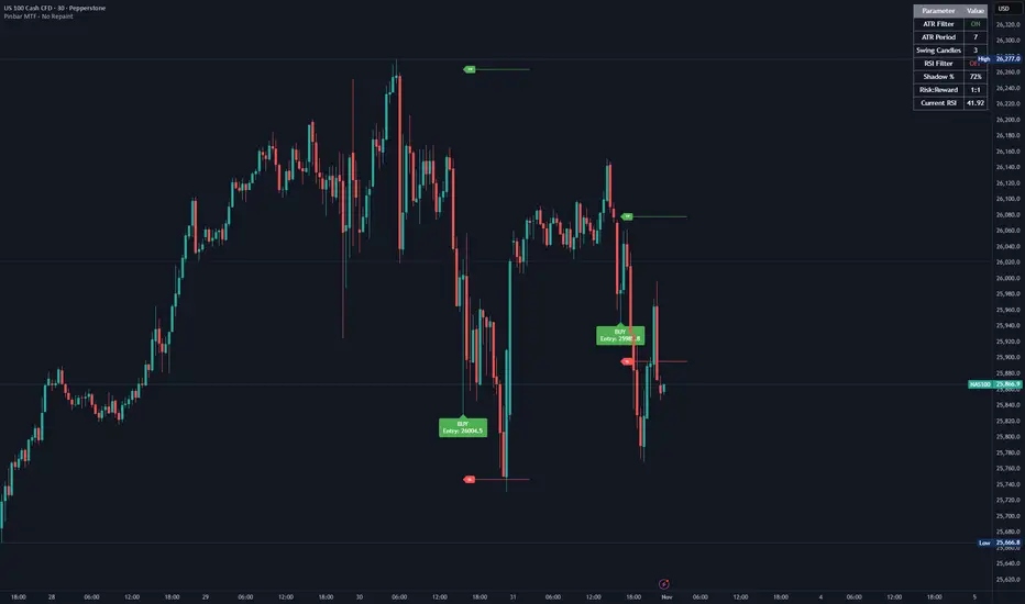
cd_correlation_analys_Cxcd_correlation_analys_Cx
General:
This indicator is designed for correlation analysis by classifying stocks (487 in total) and indices (14 in total) traded on Borsa İstanbul (BIST) on a sectoral basis.
Tradingview's sector classifications (20) have been strictly adhered to for sector grouping.
Depending on user preference, the analysis can be performed within sectors, between sectors, or manually (single asset).
Let me express my gratitude to the code author, @fikira, beforehand; you will find the reason for my thanks in the context.
Details:
First, let's briefly mention how this indicator could have been prepared using the classic method before going into details.
Classically, assets could be divided into groups of forty (40), and the analysis could be performed using the built-in function:
ta.correlation(source1, source2, length) → series float.
I chose sectoral classification because I believe there would be a higher probability of assets moving together, rather than using fixed-number classes.
In this case, 21 arrays were formed with the following number of elements:
(3, 11, 21, 60, 29, 20, 12, 3, 31, 5, 10, 11, 6, 48, 73, 62, 16, 19, 13, 34 and indices (14)).
However, you might have noticed that some arrays have more than 40 elements. This is exactly where @Fikira's indicator came to the rescue. When I examined their excellent indicator, I saw that it could process 120 assets in a single operation. (I believe this was the first limit overrun; thanks again.)
It was amazing to see that data for 3 pairs could be called in a single request using a special method.
You can find the details here:
When I adapted it for BIST, I found it sufficient to call data for 2 pairs instead of 3 in a single go. Since asset prices are regular and have 2 decimal places, I used a fixed multiplier of $10^8$ and a fixed decimal count of 2 in Fikira's formulas.
With this method, the (high, low, open, close) values became accessible for each asset.
The summary up to this point is that instead of the ready-made formula + groups of 40, I used variable-sized groups and the method I will detail now.
Correlation/harmony/co-movement between assets provides advantages to market participants. Coherent assets are expected to rise or fall simultaneously.
Therefore, to convert co-movement into a mathematical value, I defined the possible movements of the current candle relative to the previous candle bar over a certain period (user-defined). These are:
Up := high > high and low > low
Down := high < high and low < low
Inside := high <= high and low >= low
Outside := high >= high and low <= low and NOT Inside.
Ignore := high = low = open = close
If both assets performed the same movement, 1 was added to the tracking counter.
If (Up-Up), (Down-Down), (Inside-Inside), or (Outside-Outside), then counter := counter + 1.
If the period length is 100 and the counter is 75, it means there is 75% co-movement.
Corr = counter / period ($75/100$)
Average = ta.sma(Corr, 100) is obtained.
The highest coefficients recorded in the array are presented to the user in a table.
From the user menu options, the user can choose to compare:
• With assets in its own sector
• With assets in the selected sector
• By activating the confirmation box and manually entering a single asset for comparison.
Table display options can be adjusted from the Settings tab.
In the attached examples:
Results for AKBNK stock from the Finance sector compared with GARAN stock from the same sector:
Timeframe: Daily, Period: 50 => Harmony 76% (They performed the same movement in 38 out of 50 bars)
Comment: Opposite movements at swing high and low levels may indicate a change in the direction of the price flow (SMT).
Looking at ASELS from the Electronic Technology sector over the last 30 daily candles, they performed the same movements by 40% with XU100, 73.3% (22/30) with XUTEK (Technology Index), and 86.9% according to the averages.
Comment: It is more appropriate to follow ASELS stock with XUTEK (Technology index) instead of the general index (XU100). Opposite movements at swing high and low levels may indicate a change in the direction of the price flow (SMT).
Again, when ASELS stock is taken on H1 instead of daily, and the length is 100 instead of 30, the harmony rate is seen to be 87%.
Please share your thoughts and criticisms regarding the indicator, which I prepared with a bit of an educational purpose specifically for BIST.
Happy trading.
